4.5. リモートコントロール

このセクションでは、リモート接続を使用して TII Spectrometry で制御される分光器からデータを記録し、表示する方法の実例を紹介します。このコードは Jupyter notebook で実行することを想定しており、matplotlib がインストールされている必要があります。

1. まず、必要なライブラリをインポートする必要があります。

   import asyncio
   import struct
   import json
   import matplotlib.pyplot as plt
   

   最後の行（matplotlib のインポート）はオプションであり、表示する場合にのみ必要です。

2. 次に、TII Spectrometry サーバーに接続します。

   host = '192.168.2.180'
   port = 4711
   
   reader, writer = await asyncio.open_connection(host, port)
   print(f"Connected to {host}:{port}")
   

   ここで、host は TII Spectrometry 分光器サーバーを実行しているマシンの IP アドレスです。これはサーバーのダイアログウィンドウ (図 2.10) に表示されます。port はサーバーのポートで、デフォルトは 4711 です。

3. データを取得するためのヘルパー関数を定義します。

   async def fetch_data(writer, reader, command):
       command = command + "\n"
       writer.write(command.encode())
       await writer.drain()
       print(f"Sent: {command}. Waiting for data...")
   
       # 3. Read the 4-byte Big-Endian Length Header
       header = await reader.readexactly(4)
       msg_len = struct.unpack('>I', header)[0]
       print(f"Header received. Expecting {msg_len} bytes of JSON data.")
   
       # 4. Read the JSON payload
       payload = await reader.readexactly(msg_len)
       data = json.loads(payload.decode('utf-8'))
   
       print("Data received successfully!")
       return data
   

   これにより以下の処理が行われます：

   • コマンドを送信する

   • サーバーからのレスポンスの最初の 4 バイトを読み取り、JSON ペイロードの長さを特定する

   • 特定した長さを使用して JSON ペイロードを読み取る

   • ペイロードを Python の辞書型にデコードする

4. このヘルパー関数を使用して、スペクトルを記録できます。

   spectrum = await fetch_data(writer, reader, "ACQUIRE")
   

   スペクトルデータには、セクション 2.1.9.2 に記載されているキーを使用してアクセスできます。例えば、以下を実行すると

   spectrum['timestamp']
   

   ノートブックにタイムスタンプが表示されます。

   '2026-03-02T17:15:18.376000+09:00'
   

5. スペクトルデータは spectrum_x および spectrum_y キーを使用してアクセスできます。matplotlib を使用してスペクトルをプロットするには、以下を使用します。

   plt.plot(spectrum['spectrum_x'], spectrum['spectrum_y'])
   plt.show()
   

   

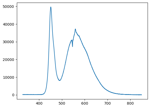
   図 4.17 matplotlib を使用したスペクトルのプロット。

6. 現在の分光器の構成を取得するには、GET_CONFIGURATION コマンドを使用します。これにより、辞書、または複数の分光器が接続されている場合は辞書のリストが返されます。

   {
       'n_average': 1,
       'spectral_domain': 1,
       'identifier': 'DS-InGaAs-256 #16052512',
       'intensity_calibration': None,
       'use_intensity_calibration': False,
       'intensity_calibration_unit': '',
       'use_nlir': False,
       'use_nlir_crop': True,
       'exposure_time': 100,
       'x_timing': 3,
       'manufacturer': 'StellarNet',
       'is_active': True,
       'use_stitching': False,
       'switchover_wl': 0
   }
   

7. データを送信するために、再度ヘルパー関数を定義します。

   async def send_data(writer, reader, command, payload):
       command = command + "\n"
       writer.write(command.encode())
   
       payload = json.dumps(payload).encode('utf-8')
       header = struct.pack('>I', len(payload))
       
       writer.write(header)
       writer.write(payload)
       await writer.drain()
   

   この関数は、command と Python の辞書または辞書のリスト形式の payload を受け取り、これらを JSON にエンコードして、長さプレフィックス付きの JSON データとして送信します。

8. この関数を使用して分光器を構成できます。

   await send_data(writer, reader, "SET_CONFIGURATION", {"n_average": 1, 'exposure_time':50})
   

   ここでは、露光時間 (exposure_time) を 50 ms に、積算回数 (n_average) を 1 に設定しています。

   リストを使用することで、複数の分光器を制御できます。

   await send_data(writer, reader, "SET_CONFIGURATION", [{"identifier": "DS-InGaAs-256 #16052512", "n_average": 1, 'exposure_time': 100, "is_active": True}])    
   

   identifier キーは必須です。

9. これにより、ループ処理などを用いて分光器を完全にプログラム制御することが可能になります。

   exposureTimes = [5,10,25,50,100,250,500,1000]
   
   for t in exposureTimes:
       await send_data(writer, reader, "SET_CONFIGURATION", {'exposure_time':t})
       sp = await fetch_data(writer, reader, "ACQUIRE")
       plt.plot(sp['spectrum_x'], sp['spectrum_y'], label=f"Exposure: {t} ms")
       await asyncio.sleep(1)
   
   plt.legend()
   plt.show()
   

   このスニペットは、異なる露光時間でスペクトルを取得し、簡単なグラフにプロットします。

   

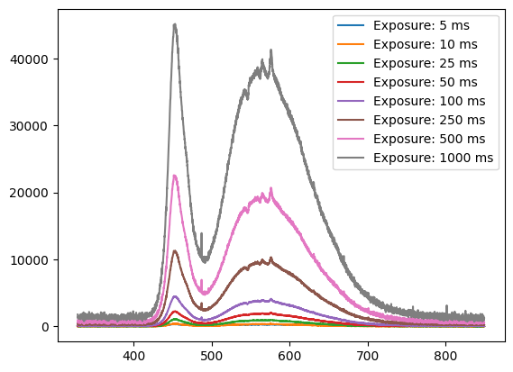
   図 4.18 matplotlib を使用したスペクトルのプロット。

10. 終了後は、接続を閉じるのが良い習慣です。

    writer.close()