3.4. Modeling

The Modeling package of TII Spectrometry allows to build and use predictive models to analyze spectral datasets. Taking spectra as the input, two different kinds of analysis are available:

• Regression Analysis: Regression is used when the output property you want to predict is a continuous numerical variable, for example concentration, quality score, temperature, or moisture level. A typical example would be concentration prediction by using the absorption spectrum of a chemical solution to predict the exact concentration of a solute, often relying on the Beer-Lambert Law.

• Classification Analysis: Classification is used when the output property you want to predict is a discrete, categorical label or class, such as material type, defect presence, or grade level. A typical example would be material identification: Classifying an unknown plastic sample as Polypropylene (PP) or Polyethylene (PE) based on its IR spectrum.

The Modeling package is can be accessed using Analysis ‣ Modeling ‣ Train/Predict and is available for any spectrometer.

See also

See the Application Example Plastic Identification to see this in action.

3.4.1. General Overview

Details on Regression and Classification analysis will be discussed in dedicated sections.

Both types of analysis, however, share a common workflow:

1. record a training dataset, e.g. spectra of known materials (for Classification) or of known concentration (for Regression).

2. build a Model using this dataset (Training): This typically involves:

   • assigning labels (numerical or categorical) to the dataset

   • preprocessing the data, e.g. by

     • Baseline Correction: Removing unwanted background signal offsets.

     • Normalization: Scaling the spectra to remove variations in overall light intensity or path length.

     • Smoothing: Reducing high-frequency noise.

     • Cropping: Remove unnecessary spectral regions.

   • training the model, e.g. using linear regression to fit a calibration curve

   • validating the model

3. once the Model has been trained, it can be used for Prediction using unknown samples. The model can also be saved to disk for later use.

Tip

Trained models can be used in TII Spectrometry in the following places:

• for real-time monitoring using both Classification and Regression models in the Monitor view.

• to extract a numerical value from spectra (using a Regression model) during time-lapse recordings

Note

In principle, signals from more than one spectrometer can be incorporated into the model, e.g. spectrometers

• covering different spectral ranges

• spectrometers measuring the same process at different locations

Note

Models, are, at least in principle, device-independent, which means that models trained on spectral datasets of one spectrometer can be used for prediction using datasets of a different device. The following caveats apply:

• spectra have to appropriately normalized to account for differences in device sensitivity (this is best practice anyway)

• spectral ranges should (roughly) coincide and, crucially, include the spectral features that are required by the model for discrimination. As a trivial example, a model trained on near-IR data will (obviously) not work when using a spectrometer operating in the visible range. For spectral ranges of suitable overlap, TII Spectrometry will use interpolation and padding to transform spectral data and account for different spectral resolutions.

3.4.2. Pre-Processing

Pre-processing involves pre-treating the data to remove noise or scattering effects. Pre-processing options are shared between regression and classification models and the same rationale applies to both types of analysis.

Note

Pre-processing settings are part of the model. They will be saved in the model file and applied to spectra during the Prediction phase.

TII Spectrometry offers the following pre-processing settings (Figure 3.11):

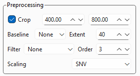
Fig. 3.11 Pre-processing Settings

Crop

Allows selecting a spectral subregion.

Baseline

Removes a non-linear baseline from the dataset using the Statistics-sensitive Non-linear Iterative Peak-clipping (SNIP) algorithm (Ryan, 1988). The Extent parameter changes the curvature of the baseline.

Note

A constant offset can easily be removed using Scaling. If the baseline can be removed by background subtraction during spectral acquisition, this is likely preferable.

Filter

Applies a convolutional smoothing filter to the data. The settings are identical to the Filter setting in the main window.

Scaling

Scales (normalizes) the data. Three options are available:

• None: Performs no scaling

• Min-Max: Scales each spectrum in the range between 0 and 1.

• SNV: Applies Standard Normal Variate scaling.

Important

Scaling is crucial for Regression or Classification performance and, in particular, to achieve generalized models that are independent of:

• illumination conditions

• spectrometer sensitivity or exposure time

See Table 3.1 for a comparison of the scaling methods of TII Spectrometry.

3.4.2.1. Scaling Methods

3.4.2.1.1. Min-Max Scaling

Min-Max scaling, also known as feature scaling or unity-based normalization, is a data preprocessing technique to transform numerical features to a specific, predefined range, usually \([0, 1]\).

For a single spectrum \(X_i\), the transformation is:

\[X_{\text{MM}, i} = \frac{X_i - \min(X_i)}{\max(X_i) - \min(X_i)}\]

Here:

• \(X_i\) is the original spectrum.

• \(\min(X_i)\) and \(\max(X_i)\) are the minimum and maximum absorbance/reflectance values within that single spectrum.

The primary goal of per-spectrum Min-Max scaling is to remove multiplicative scaling differences caused by factors like changes in path length, sample packing, or light source intensity that affect the magnitude of the spectrum.

• Baseline Anchor: This method forces the lowest point in the spectrum to \(0\) and the highest point to \(1\). This effectively corrects for differences in the dynamic range or overall spread of the signal intensity from one sample to the next.

• Contrast Preservation: It preserves the relative shape and proportionality of the spectral features, ensuring that the height ratios between peaks remain consistent.

3.4.2.1.2. Standard Normal Variate Scaling

SNV scaling is a per-spectrum operation, meaning it is applied independently to each individual spectral curve in a dataset. It is a two-step process that normalizes the spectrum based on its own mean and standard deviation. The Standard Normal Variate (SNV) scaling method is a common technique used in spectroscopy, particularly with Near-Infrared (NIR) data, to perform baseline correction and standardize spectral features. For a single spectrum \(X_i\) (a vector of measured values at different wavelengths), the transformation to the scaled spectrum \(X_{\text{SNV}, i}\) is given by:

\[X_{\text{SNV}, i} = \frac{X_i - \overline{X}_i}{s_i}\]

Here:

• \(X_i\) is the original spectrum.

• \(\overline{X}_i\) is the mean of all absorbance/reflectance values within that spectrum.

• \(s_i\) is the standard deviation of all absorbance/reflectance values within that spectrum.

This formula results in a new spectrum where the average intensity is centered near zero, and the variance (spread) is standardized to one.

SNV scaling effectively removes two major sources of variation that are not related to the sample’s chemical composition:

1. Baseline Offset (Additive Effects): The subtraction of the mean (\(\overline{X}_i\)) corrects for constant vertical shifts in the spectrum caused by factors like changes in the sample path length or light scattering variations that affect the overall intensity level equally across all wavelengths.

2. Scaling Differences (Multiplicative Effects): Dividing by the standard deviation (\(s_i\)) corrects for variations in the slope or overall magnitude of the spectrum caused by differences in scattering properties, particle size, or instrument changes.

By removing these physical variations, SNV enhances the spectral features that are genuinely related to the chemical composition (the characteristic absorption peaks), making subsequent modeling more accurate and robust.

Table 3.1 Min-Max vs. SNV

Feature	Per-Spectrum Min-Max Scaling	Standard Normal Variate (SNV)
Centering Reference	The absolute minimum value of the spectrum.	The mean value (\(\overline{X}_i\)) of the entire spectrum.
Scaling Reference	The range (\(\max - \min\)) of the spectrum.	The standard deviation (\(s_i\)) of the spectrum.
Targeted Error	Primarily Multiplicative scaling (intensity differences).	Both Additive baseline shifts and Multiplicative scaling.
Effect on Peaks	Anchors the lowest point to 0 and stretches/compresses the peaks to fit between 0 and 1.	Centers the whole spectrum around 0, making the negative and positive peak areas equivalent in deviation.

See also

See the Application Example Plastic Identification for a discussion of data preprocessing in the context of a pratical application.

3.4.3. Regression Analysis

As discussed above, Regression involves assigning numerical values to spectra.

TII Spectrometry offers two different methods to train Regression models (Table 3.2):

• manual training using linear regression. This requires the selection of a relevant spectral feature, e.g. the area of a peak or the intensity ration of two peaks, from which a calibration curve is constructed. Prediction is performed using this calibration curve.

• semi-automated, machine-learning based regression based on Support Vector Regression (SVR). In contrast linear regression, which try to minimize the sum of squared errors, SVR tries to fit the best line or hyperplane while ensuring that most of the predicted data points are within a certain distance of that line. For non-linear relationships (which are common in spectral datasets), SVR uses the Kernel Trick (e.g., the Radial Basis Function or RBF kernel) to map the input features into a higher-dimensional space where a linear hyperplane can successfully model the non-linear relationship in the original space. This method is not only robust to noise and outliers but also can model complex, non-linear relationships between spectral features and continuous properties (like concentration or quality scores) using kernels. In contrast to linear regression, no feature selection by the user is required.

Table 3.2 Linear Regression vs. SVR

Feature	Linear Regression	Support Vector Regression (SVR)
Model Type	Parametric (Assumes a linear relationship).	Non-Parametric (Flexible, often uses kernels).
Objective Function	Minimizes the Sum of Squared Errors (SSE), penalizing all errors equally.	Minimizes the errors that fall outside a defined margin (\(\epsilon\)), ignoring small errors within the margin.
Error Treatment	Sensitive to all data points and outliers, especially those far from the line.	Insensitive to data points within the \(\epsilon\)-tube; robust to noise and outliers.
Model Complexity	Simple, easy to interpret, fast to train.	More complex, computationally intensive, especially with kernel methods.
Non-Linearity	Cannot model non-linear relationships without manual feature engineering (e.g., polynomial terms).	Naturally handles non-linear relationships using the Kernel Trick (e.g., RBF kernel).
Key Points	Finds the line that best fits the average of the data.	Finds the line that best fits the boundary defined by the Support Vectors.
Application Suitability	Simple, well-behaved datasets where relationships are known to be linear.	High-dimensional, complex datasets (like spectral data) where non-linear modeling and noise robustness are required.

3.4.3.1. Training

3.4.3.1.1. Linear Regression

The Train view (Analysis ‣ Modeling ‣ Train/Predict, Figure 3.12) contains the following user interface elements:

• the spectra sidebar on the left, which contains the spectra used for training as well as their labels

• the spectrum view, which contains the spectra after pre-processing

• the parameter sidebar on the right, which controls pre-processing and training settings

• the result view (center bottom), which contains the calibration curve and the predicted numerical value for each training spectrum.

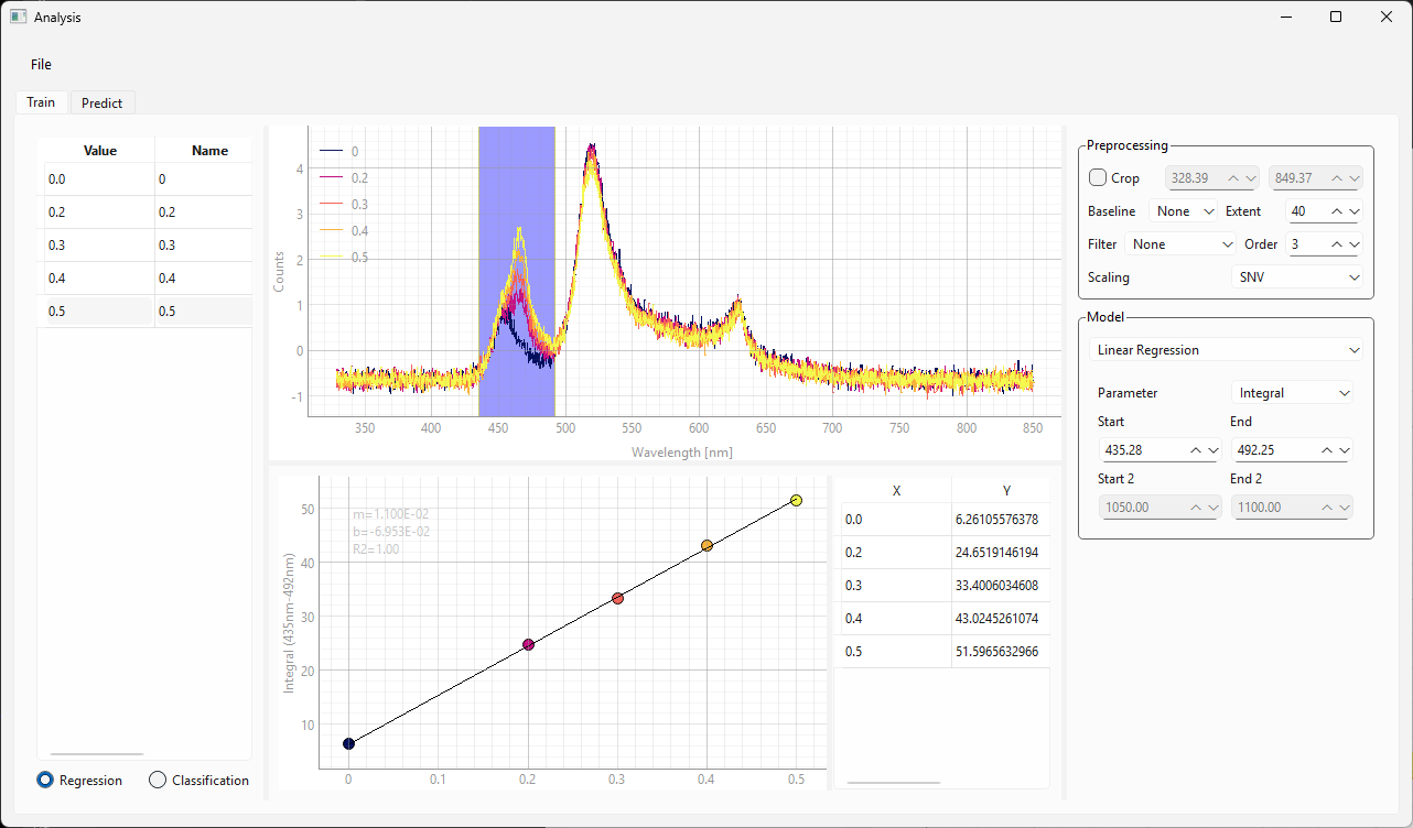
Fig. 3.12 The Training view of the Modeling Window

To train a Regression Model:

1. display the Modeling window using Analysis ‣ Modeling ‣ Train/Predict (Figure 3.12).

2. select the Train tab (the Train tab is shown in Figure 3.12).

3. select Regression from the radio button set below the left sidebar

4. load a dataset. This can be done by:

   • dragging spectra from the spectra side bar into the left sidebar of the Modeling window

   • dragging a saved file (in .hdf5 format) onto the left sidebar

   The spectra contained in the file will now appear in the sidebar and the spectrum view

5. apply numerical labels to each spectrum. This can be done by:

   • double-clicking on the cell in the Value column

   • entering a numerical value, e.g. a concentration

   Hint

   Since labeling can be tedious, labeled datasets can be saved using File ‣ Save Dataset.

6. select appropriate pre-processing parameters.

   Tip

   The spectra in the spectra view will reflect the current preprocessing settings.

   For the data in Figure 3.12 in we have :

   • cropped the spectral range between 400 and 800 nm

   • applied SNV scaling

   Important

   Scaling is generally recommended for satisfactory model performance. Please see the discussion in Section 3.4.2.1 for details.

See also

For this example, we are training a linear regression model, which requires manual feature selection. For training a Support Vector Regression model, jump forward to Section 3.4.3.1.2.

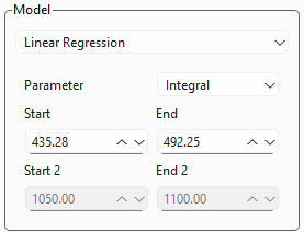
Fig. 3.13 Linear Regression Settings

7. Figure 3.13 displays the settings for a linear regression analysis.

   • Parameter: Allows the selection of a spectral parameter, e.g. an integral, peak width, or peak area ratio. Please see Section 3.1 for available parameters and their definition.

   • Start and End determine the spectral range from which the parameter is computed. This parameter can also be adjusted by dragging and resizing the region selector in the spectrum view.

   • for peak ratios, the Start 2 and End 2 settings will become available

8. The Calibration Curve (bottom of Figure 3.12) will reflect the settings. Adjust settings until the linear trendline matches the data.

   • the table adjacent to the calibration curve shows the X and Y values of the curve

   • slope, y-intercept, and \(\rm{R}^2\) value are displayed in the calibration curve graph

9. If you are satisfied with the model, switch to the Predict tab (Section 3.4.3.2).

10. (optional) Save the model to disk using File ‣ Save Model.

3.4.3.1.2. Support Vector Regression

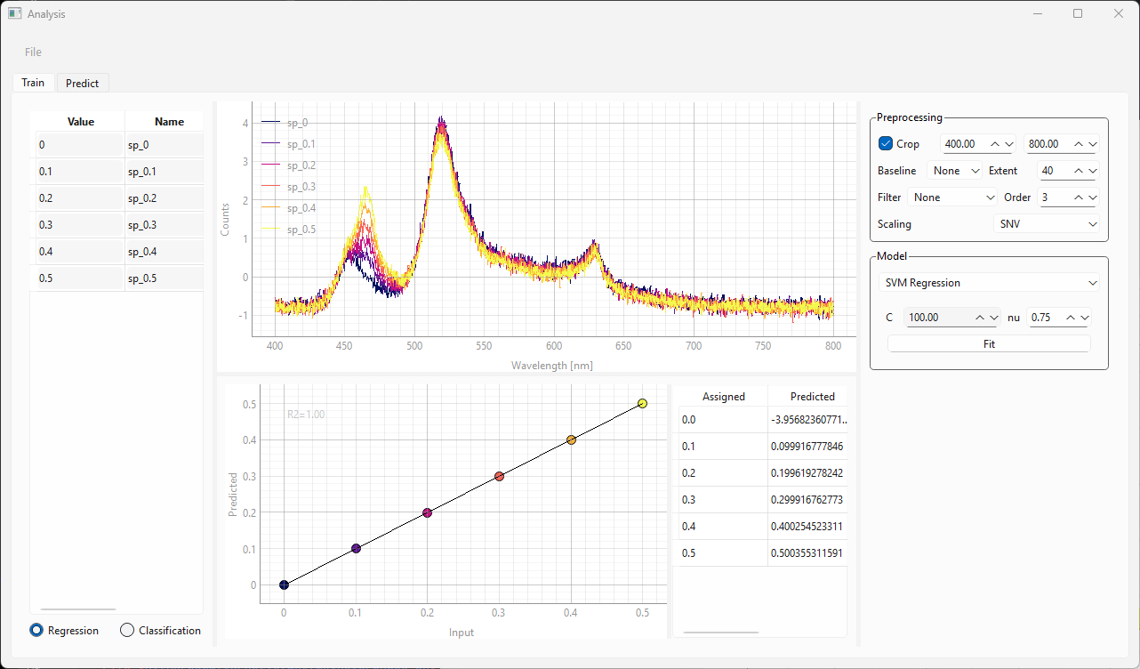
Fig. 3.14 The Training view of the Modeling Window (SVR)

Loading data, assigning labels, and preprocessing are identical between linear regression and SVR models (steps 1-6 in Section 3.4.3.1.1).

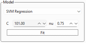
Fig. 3.15 SVR Settings

Figure 3.15 shows a close-up of the SVR settings box, which has two parameters:

C

The parameter \(C\) controls the trade-off between model complexity and the degree of tolerance for training errors.

• A small \(C\) means a weak penalty. The model allows more points to violate the margin, resulting in a smoother, simpler hyperplane (higher bias, lower variance). This is often desired if the data is very noisy.

• A large \(C\) means a strong penalty. The model tries hard to include almost all training points within the margin, resulting in a more complex, wiggly hyperplane (lower bias, higher variance). This can lead to overfitting if the data is noisy.

\(\nu\) (Nu)

\(\nu\) places an upper bound on the fraction of training errors (outliers that fall outside the margin) and a lower bound on the fraction of Support Vectors relative to the total number of training points. \(\nu\) must be between 0 and 1. \(\nu\) implicitly determines the value of \(\epsilon\), which is used in some SVM implementations.

• A small \(\nu\) (e.g., 0.1): Allows for a tighter margin and fewer outliers. This corresponds to the model being more restrictive, similar to a high \(\epsilon\)

• A large \(\nu\) (e.g., 0.9): Allows for a wider margin and more potential outliers/Support Vectors.

Fit

Click the Fit button to train the model. This will update the result graph and result table.

The SVR algorithm automatically extracts the relevant spectral features for regression from the dataset. The resulting curve is shown in at the bottom of the Train window. The curve displays the assigned (Input) vs Predicted numerical value - ideally this should be a straight line with slope 1 and datapoints should coincide with the black line. The table on the right side of the graph displays the numerical values of the assigned labels.

3.4.3.2. Prediction

To use a model, select the Predict tab (Figure 3.16).

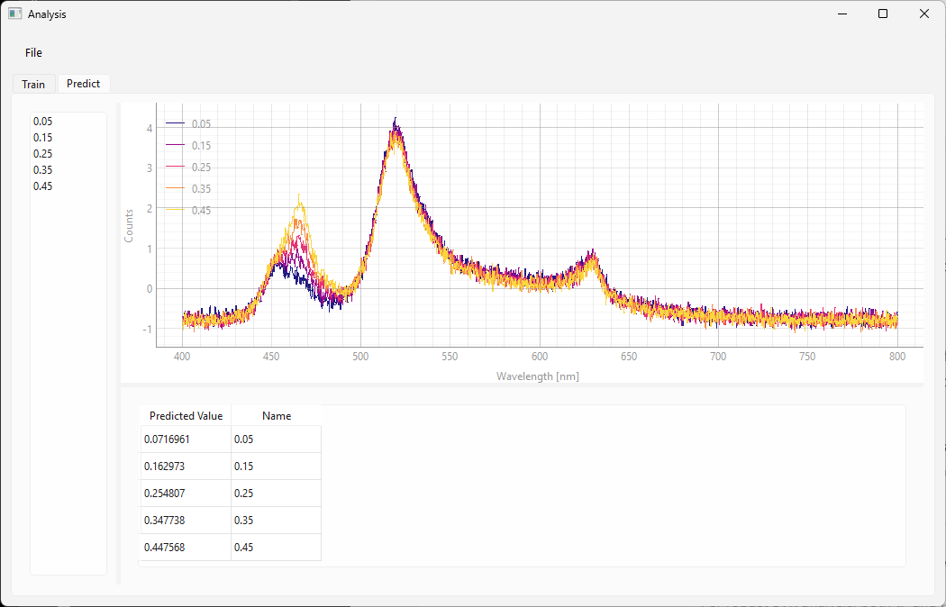
Fig. 3.16 The Predict screen (SVR)

The Predict tab will contain the last trained model from the Train tab. Alternatively, you can load a model from disk using File ‣ Load Model.

Tip

You can switch back and forth between the Train and Predict screens to optimize model training using cross-validation.

To use a model:

1. load data by dragging a .hdf5 file onto the left sidebar. This will:

   • open the spectra

   • apply the processing selected in the model

   • perform the regression analysis

2. the results can be found in the table at the bottom. It contains:

   • the predicted numerical value

   • the name of the spectrum

In the example in Figure 3.16, the spectra were recorded at known concentrations so this dataset can be used for validation. The concentrations in the validation dataset are different from the concentrations employed during training. The Name column contains the (known) correct value of the predicted parameter. It can be seen that the agreement between predicted and correct validation value is very good, which indicates that we have successfully trained the model.

Note

For linear regression models,

• the result table in the Predict screen also contains the extracted spectral parameter (e.g. integrated peak are) in the Y column

• the Predict screen displays the calibration curve and the position of the of the samples on the curve.

See Figure 3.17 for an example.

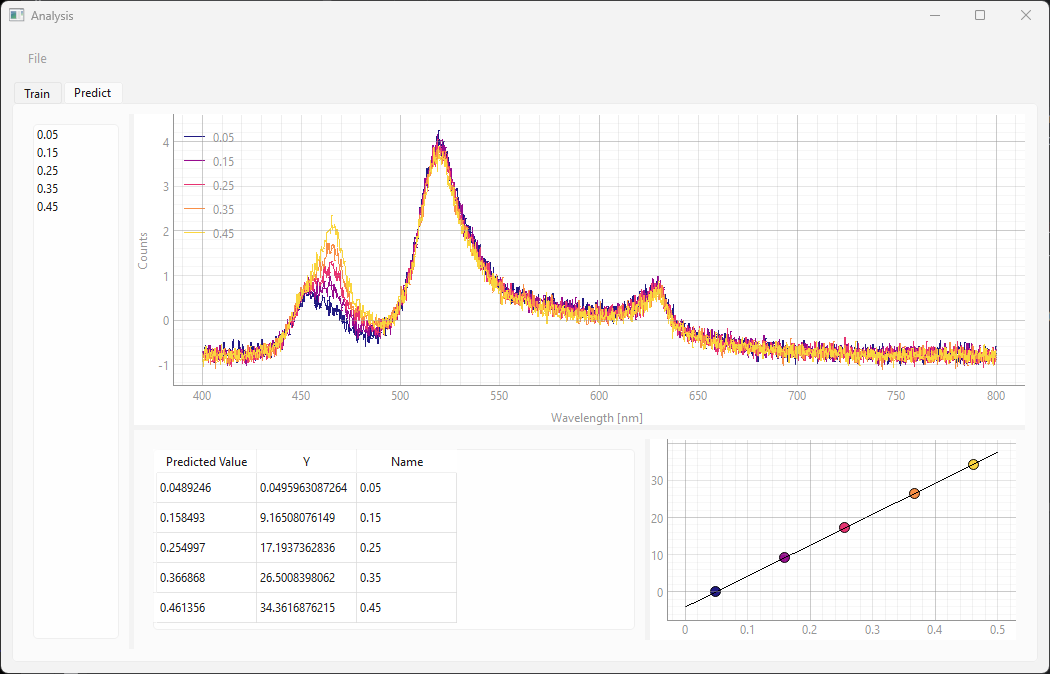
Fig. 3.17 The Predict screen (Linear Regression)

3.4.4. Classification Analysis

For Classification, TII Spectrometry offers Support Vector Machine (SVM) Classification. Analogous to Support Vector Regression (SVR), the goal of SVM classification is to find the hyperplane that has the largest margin between the nearest training data points of any class.

See also

Many of the remarks on Support Vector Regression also apply to SVM classification.

3.4.4.1. Training

Training a Classification model generally mirrors the steps laid out in Section 3.4.3.1.1:

1. display the Modeling window using Analysis ‣ Modeling ‣ Train/Predict (Figure 3.18).

2. select the Train tab (the Train tab is shown in Figure 3.18).

3. select Classification from the radio button set below the left sidebar

4. load a dataset.

5. apply labels to the dataset. Labels can any text.

   Tip

   Labeled datasets can be saved to disk

6. adjust the SVM hyperparameters \(C\) and \(\nu\) (Section 3.4.3.1.2) and click Fit to train the model.

7. the result view at the bottom shows the confusion matrix, which plots the predicted vs. assigned label. Ideally, all values fall on the diagonal.

8. if you are satisfied with the model, switch to the Predict tab.

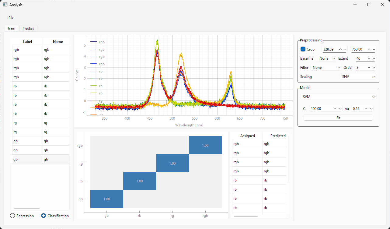
Fig. 3.18 Training a Classification model.

3.4.4.2. Prediction

Using a trained classification model for prediction mirrors the use of regression models.

Simply:

1. Load a dataset by dropping a .hdf5 file onto the left sidebar.

2. The classification result will be shown in the table at the bottom (Figure 3.19)

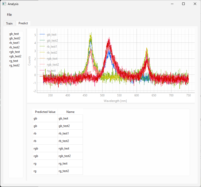
Fig. 3.19 Using a Classification model.

For the dataset in Figure 3.19, the first part of the name of the spectra used for prediction contains the correct label. It can be seen that the agreement of the predicted value with the correct label is excellent.

3.4.5. Monitoring

You can use trained models (both Classification and Regression models) in TII Spectrometry for real-time monitoring, for example:

• to monitor a concentration using a Regression model

• to identify different substances

This functionality can be accessed using Analysis ‣ Modeling ‣ Monitor to show the Monitoring screen (Figure 3.20). Here,

• you can load a model using the Load button

When using the spectrometer in single or continuous acquisition mode, the prediction result of the selected model for the currently acquired spectrum will be shown in the top right.

Important

The prediction results are only displayed but not saved to disk. To record prediction results, use a time-lapse acquisition.

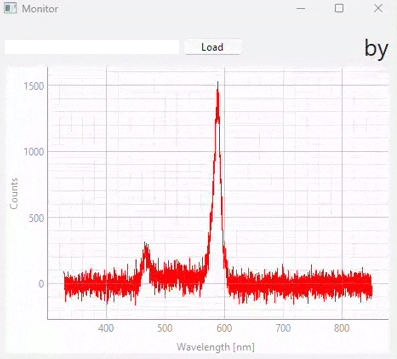
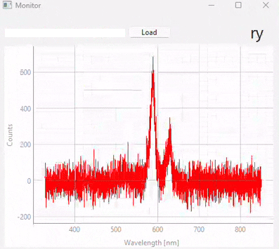
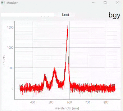
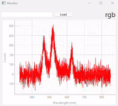
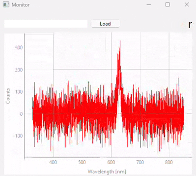
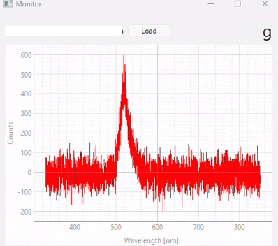
Fig. 3.20 Real-time monitoring (snapshots)

Figure 3.20 displays snapshots of the prediction result at different points in time. The dataset / model used in this experiment (which contains many different sample classes) is displayed in Figure 3.21. It is important to note that:

• the signal-to-noise ratio of the test spectra (during monitoring) is a lot lower than the SNR of the spectra used for training. Due to appropriate scaling and the relatively noise-tolerant SVM model, this has no detrimental effect during the prediction stage.

• prediction fidelity is excellent - there are no misclassifications

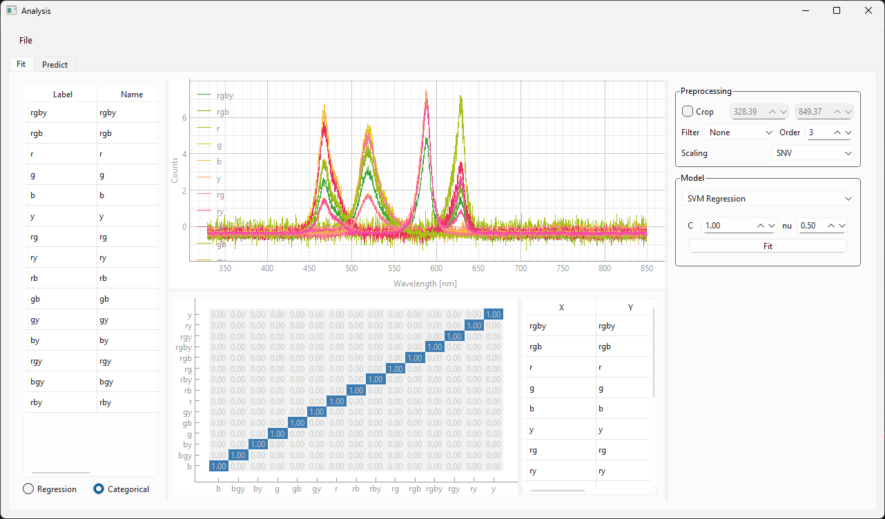
Fig. 3.21 The Classification model used for the monitoring experiment.