5.1. Fast Fourier Transform (FFT) Applied to FTIR Data

This section explains - mostly for educational purposes - how to extract spectra from space or time-domain interferogram data from a Fourier Transform Infrared spectrometer.

Figure 5.1 (left) displays a double-sided interferogram. The x-axis displays the optical path difference (OPD) - the travel distance of the interferometer’s mirrors in meters. The right panel displays the shows burst around the region of zero OPD, where maximum interference is produced by the instrument.

Note

This is the data as delivered by an ARCoptix FTIR instrument.

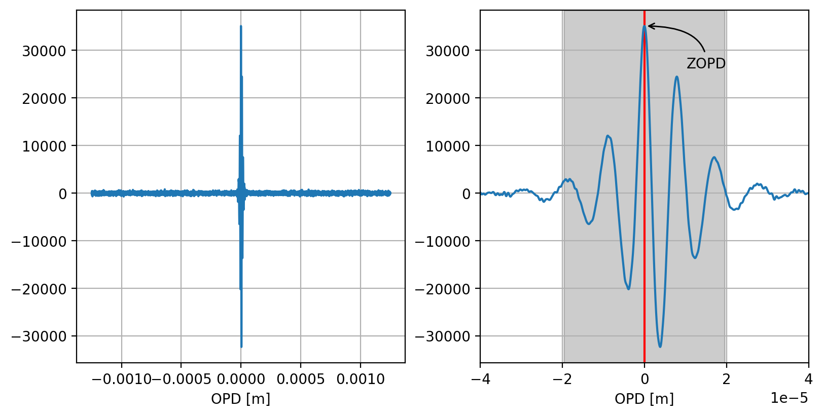
Fig. 5.1 Interferogram (left) and zoom into the ZOPD region (right)

Extracting spectral information from this data involves the following steps:

1. (optional) padding the interferogram. Padding in the space domain is equivalent to interpolation in the wavenumber domain and can be done to increase the spectral resolution.

2. preparing phase-correction data

3. extracting the sample spectrum from the phase-corrected interferogram

4. (optional) calculating absorption or transmission spectra using reference spectra

The spectrum, \(B(\nu)\), is obtained by taking the complex Fourier Transform of the interferogram, \(I(\Delta)\):

\[B(\nu) = \int_{-\infty}^{+\infty} I(\Delta) e^{-i 2 \pi \nu \Delta} d\Delta\]

Where:

• \(I(\Delta)\) is the interferogram as a function of optical path difference (\(\Delta\)).

• \(\nu\) is the wavenumber.

5.1.1. Phase Correction

In an ideal Fourier Transform (FT) system, the interferogram (the raw signal collected by the detector) should be perfectly symmetric around the Zero Path Difference (ZOPD) point, which is where the two optical paths in the interferometer are exactly equal. However, real-world FTIR instruments introduce phase errors (\(\theta(\nu)\)) due to several factors, primarily:

• Instrumental imperfections: The optical components (like the beamsplitter material) have wavelength-dependent refractive indices (dispersion), which means different wavelengths travel through the material at slightly different speeds.

• Sampling/Electronics: Minor offsets between the ZPD and the first data point recorded, or electronic filtering effects.

The phase correction method used here is the Mertz method, a multiplicative correction method that works in the frequency (wavenumber) domain. It estimates the phase error and then removes it from the full measured spectrum.

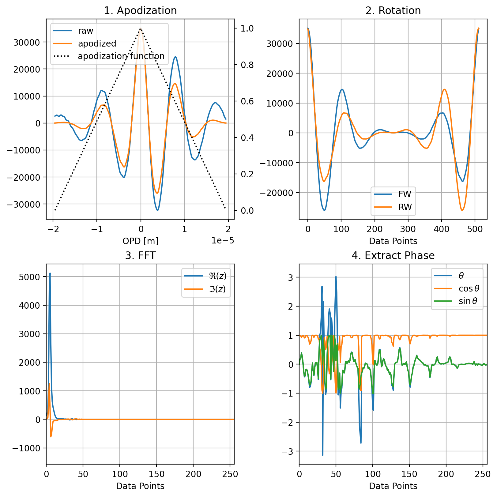
Fig. 5.2 Phase Correction

The method relies on the assumption that the instrumental phase \(\theta(\nu)\) is a slowly varying function of the wavenumber. This allows the phase to be accurately determined from a small, highly symmetric region of the interferogram around the center burst (ZOPD) where the signal-to-noise ratio is highest (gray shaded region in Figure 5.1).

• extract a small region centered on the ZOPD (Figure 5.2) \(I_{short}(\Delta)\)

• apodize this region to avoid edge effects. Here, this is done using a triangular function to yield \(I'_{short}(\Delta)\)

• rotate the data to shift ZOPD data to 0

• perform the Fourier transform (FFT)

• The resulting complex spectrum is used to calculate the phase spectrum, \(\theta(\nu)\), using the relationship between the real and imaginary parts:

  \[ \theta(\nu) = \arctan \left( \frac{\Im(z)}{\Re(z)} \right) \]

  where \(z\) is the complex Fourier transform of \(I'_{short}(\Delta)\)

5.1.2. Extracting the Sample Spectrum

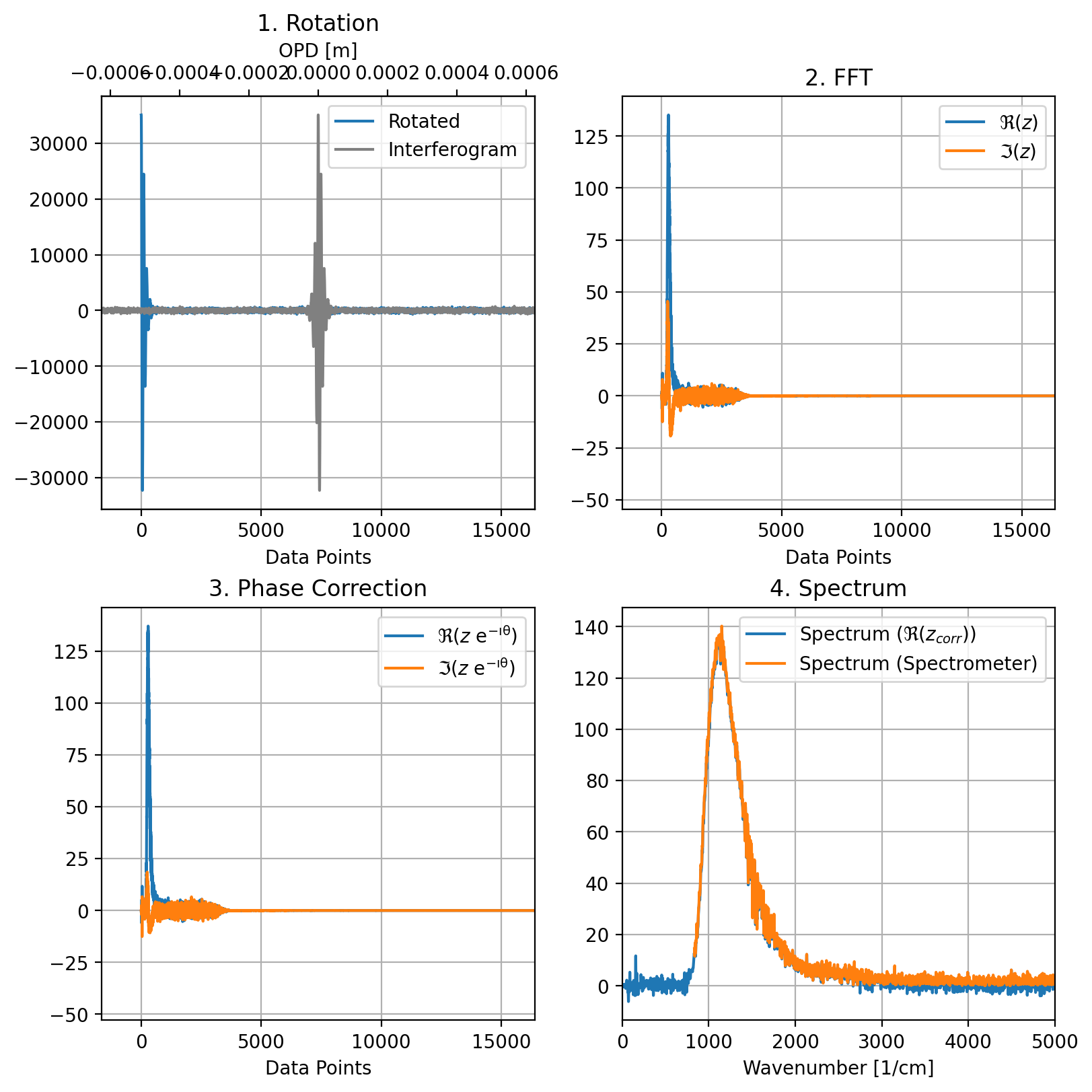
Fig. 5.3 Extracting the Spectrum

Once we have obtained the phase \(\theta(\nu)\), we can phase correct the full spectrum. To this end:

• the phase spectrum \(\theta(\nu)\) is interpolated to the full resolution of the final desired spectrum.

• the full interferogram is rotated to shift the ZOPD data to bin 0

• the FFT is applied to the rotated data

• the final phase correction is applied by multiplying the complex Fourier Transform of the full, single-sided interferogram by a correction term:

  \[ B_{corrected}(\nu) = B_{full}(\nu) \cdot e^{-i \theta(\nu)}\]

• the spectrum is the real component \(\Re(B_{corrected}(\nu))\)

Figure 5.3 panel 4 compares the spectrum extracted by this method (blue) and the spectrum obtained by the spectrometer (orange). While the overall shape is similar, the intensity is different. This is due to the fact that the spectrometer uses zero-padding by a factor of two to improve the spectral resolution. Since the FFT is scaled by \(\rm{1/n}\), this will affect the amplitude as well.

5.1.3. Results

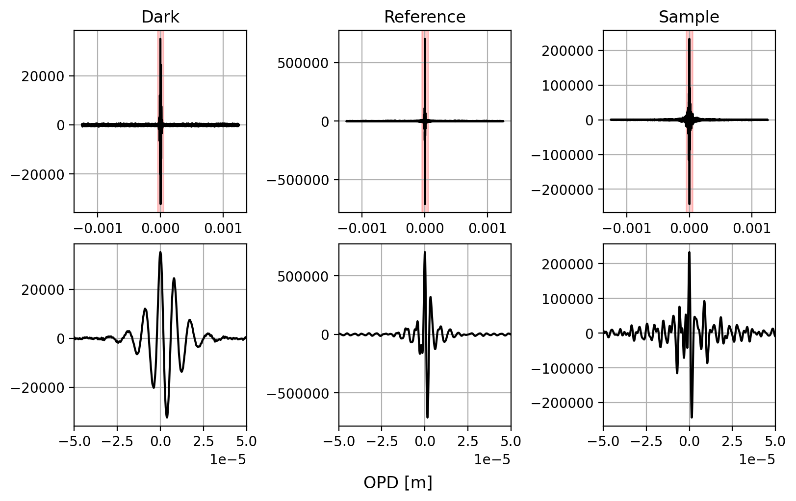
Fig. 5.4 Sample Interferograms

Figure 5.5 compares spectra that were manually extracted from interferograms (Figure 5.4) with the spectrometer’s data processing. Three spectra are shown:

• a dark spectrum where no light hits the detector

• a reference spectrum of air

• a sample spectrum of a fairly thick polystyrene sample

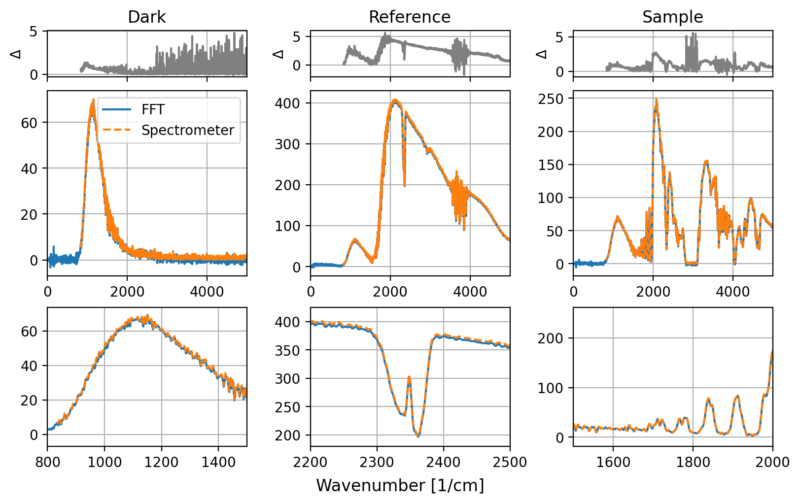
Fig. 5.5 Interferogram Analysis

For analysis:

• data was zero-padded by a factor of 2

• phase correction data prepared as laid out in Section 5.1.1

• the full interferogram was Fourier-transformed, phase corrected, and the spectrum computed from the real component.

Overall, the agreement between manual processing and the spectrometer’s result is very good. The residuals (differences between the spectra obtained by the two methods, top row of Figure 5.5) are typically very small - only a few percent of the total signal strength. Larger differences occur in regions where count rates are very low, for example in the dark spectrum at wavenumbers > 3000 cm^-1 or for the polystyrene sample between 2800 and 3200 cm^-1.

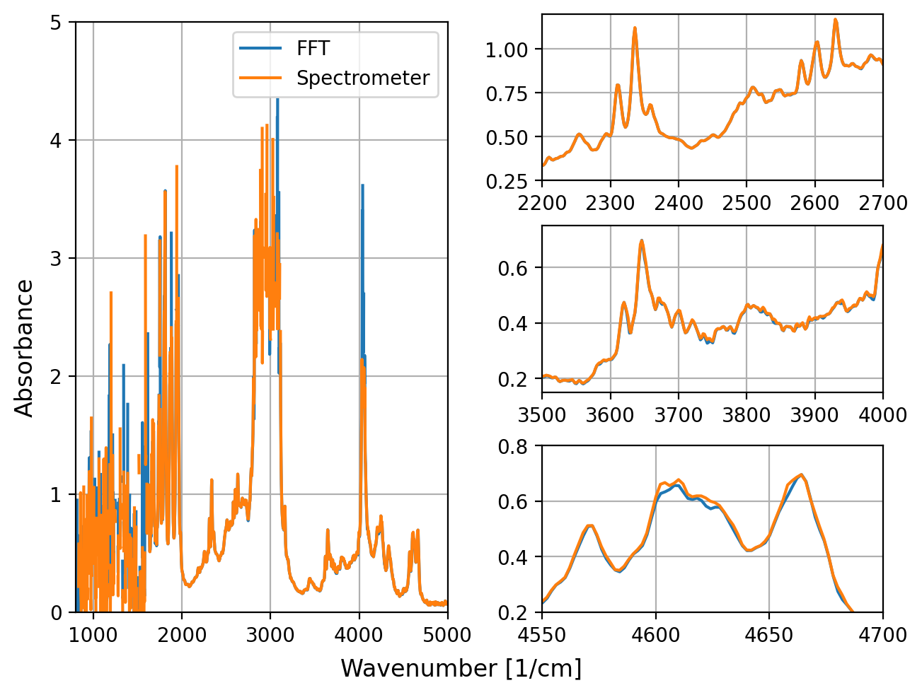
Fig. 5.6 Absorbance Spectra

Figure 5.6 shows an absorbance spectrum \(\rm{A(\nu)}\) calculated from the raw data

\[ A(\nu) = -\log_{10}{\frac{I_S(\nu) - I_B(\nu)}{I_R(\nu) - I_B(\nu)}} \]

where:

• \(\rm{I_S(\nu)}\) is the sample spectrum

• \(\rm{I_R(\nu)}\) is the reference spectrum

• \(\rm{I_B(\nu)}\) is the background (dark count) spectrum

Again, agreement is very good except for regions of high absorbance. In these regions, even small numerical differences will be emphasized due to division and application of the logarithm. The right panels of Figure 5.6 show a comparison of key spectral regions - generally, agreement is excellent.

5.1.4. An Annotated Example

This section contains Python sample code to perform interferogram analysis. It assumes that numpy is available.

5.1.4.1. Loading CSV Data

This snippet loads .csv data into the opd and y numpy arrays.

data_sp = np.loadtxt("data.csv", skiprows=1, delimiter=',')
opd, y =  data_sp[:, 0], data_sp[:, 1]

5.1.4.2. Padding

Here, we (optionally) pad the data by fillFactor. This is equivalent to increasing the scan range, hence the opd array now is a array of twice the number of points with twice the range. The y intensity data is padded symmetrically by appending zeros to the start and end.

opd = opd * fillFactor
opd = np.linspace(opd.min(), opd.max(), len(opd) * fillFactor)
y = np.pad(y, pad_width=(int((fillFactor - 1) / 2 * len(y)),), mode='constant')

5.1.4.3. Phase Extraction

First, we obtain the index of the ZOPD.

Next,

• we use a 512 point window to extract a small region around the ZOPD yShort

• we use triangular apodization to prepare y_apo

• we rotate the ZOPD bin to 0 using np.roll

• we compute the FFT using np.fft and compute the phase theta using the atan2 function

max_Y = np.argmin(np.abs(opd))

winSize = 512
xShort = np.arange(0, winSize)
yShort = y[max_Y - winSize//2 :max_Y + winSize//2]

apo_short = triangularApodization(yShort)
y_apo = yShort * apo_short
y_short_apo_rot = np.roll(y_apo[::1], winSize//2)
fft_short = np.fft.fft(y_short_apo_rot, norm='forward')
theta = np.atan2(fft_short.imag, fft_short.real)

5.1.4.4. Calculating the Spectrum

First, we interpolate the phase information to the full length of the (padded) spectrum.

theta_full = np.interp(np.linspace(xShort[0], xShort[-1], len(opd)), xShort, theta)

Next, we calculate the spectrum:

• use np.roll to rotate

• perform the FFT

• apply the phase correction by multiplying the real part of the FFT by \(\exp(- i\theta(\nu))\)

• calculating the spectrum yy as the real part of the phase corrected component.

• truncate this to the length of half of the OPD since (after phase correction) the spectrum is now symmetric

#alternatively, apply apodization here, eg
#y_apo = y * triangularApodization(y)
y_apo = y 
y_full_apo_rot = np.roll(y_apo[::1], -max_Y)
fft_full = np.fft.fft(y_full_apo_rot, norm='forward')

yy = (fft_full * np.exp(-complex(0,1)*theta_full)).real[0:len(xx)]

5.1.4.5. Calculating the Wavenumber Axis

Finally, we need to calculate the wavenumber axis. First, we calculate the wavenumber increment dx in cm^-1 and fill a numpy array xx using dx as the step size.

dx = 1/(opd.max() + np.abs(opd.min())) / 100 
xx = np.linspace(0, len(opd)//2 * dx, len(opd)//2)

5.1.4.6. Apodization

A triangular apodization function for data y can be calculated using the following function

def triangularApodization(y:np.ndarray):
    max_Y = np.argmax(y)
    x = np.arange(0, len(y))
    apo = 1-np.abs(x - max_Y) / (1 * len(x[max_Y:])) 
    apo[apo < 0] = 0
    return apo

Alternatively,

• the Norton-Beer package contains a number of functions commonly used in FTIR analysis

• standard windowing functions (Hanning etc.) will work as well.