3.3. Radiometry#
Unlike Colorimetry, which deals with the analysis of colors that originate from the changes to the spectrum of a light source (‘illuminant’) by absorption or scattering of a sample, radiometry involves the characterization of the light source itself. The Radiometry window (Figure 3.7), which can be accessed using , provides the following functionality:
measurement of the physical energy emitted by a light source in Watts
measurement of the perceived brightness of visible light (Lumens). Here, we are taking radiometric data and weighting it according to the standardized human eye sensitivity curve (V(\(\lambda\))).
Important
For the computed values of energy or brighntess to be physically meaningful, the spectrometer has to be calibrated using a light source with
a known spectrum
a known power output
To minimize geometric effects, the collection setup has to be carefully considered, for example by using an integrating sphere.
For qualitative comparison of light sources and their quality, omitting this calibration step is possible as long as the sensitivity curve of the spectrometer does not result in spectral distortion in the visible range.
characterization of light source color rendering quality from the spectral power distribution (spectrum), e.g. color temperature (CCT) or color rendering index (CRI)
See also
See Section 4.3 - Radiometric Analyis of Light Sources to see this in practice.
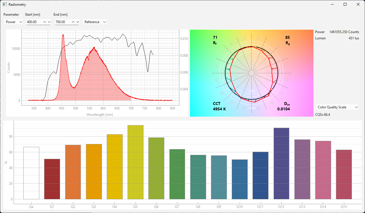
Fig. 3.7 The Radiometry window#
The Ratiometry window (Figure 3.7) hosts the following controls / UI elements (from top to bottom):
the spectrum view
3.3.1. The Settings Bar#
The Settings bar offers the following settings:
- Parameter
switches between Power (emitted energy) and Lux (perceived brightness) (Figure 3.8). To compute the perceived brightness, the spectrum is multiplied by a standardized human eye sensitivity curve V(\(\lambda\)), which is centered around 550 nm.
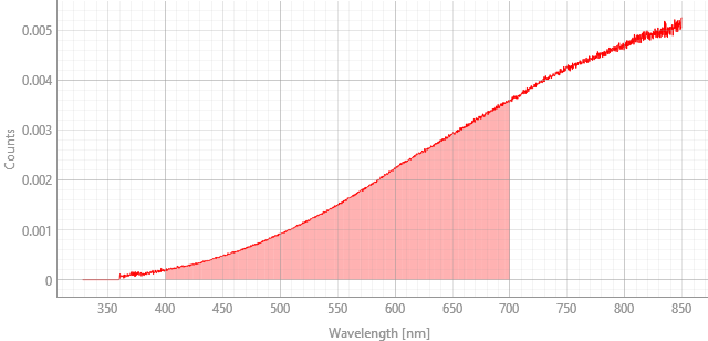
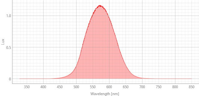
Fig. 3.8 Energy vs perceived brightness#
- Start
The lower spectral bound used to determine the emitted power
- End
The upper spectral bound used to determine the emitted power
Hint
The area used for integration is indicated by the shaded region in the spectrum view.
- Accessory Display
Toggles the (optional) display of either:
the reference illuminant used for calculating the color fidelity index \(R_f\) and the color gamut index \(R_g\). For a color temperature (CCT) < 5000 K, a theoretical Planckian (black-body) radiator at that CCT will be used, for higher color temperatures, the CIE Daylight distribution will be used. See Figure 4.7 for further examples of reference illuminants.
the raw spectral data (before intensity calibration)
Hint
Displaying the raw spectral data can be useful to judge how much of the dynamic range of the spectrometer is actually used and to optimize acquisition parameters to obtain a high-signal-to-noise ratio while avoiding saturating the detector.
3.3.2. The IES TM-30-18 Color Vector Graphic#
The Color Vector Graphic translates the numerical color quality data of a light source derived from its spectral power distribution (SPD) into a visual map of color shifts. The graphic is a circular plot that visually represents how a test light source changes the hue and saturation of colors compared to an ideal reference source (like daylight or a black-body radiator). It is divided into 16 hue bins (sections around the circle), which makes it easy to identify deficiencies or enhancements in specific color ranges (Figure 3.9).
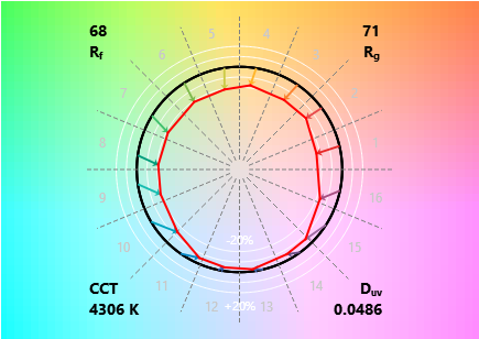
Fig. 3.9 The Color Vector Graphic#
This plot shows:
- The Reference Ring
The central black circle in Figure 3.9 represents the chromaticity coordinates of the 99 Test Color Samples (TCSs, also see Section 3.3.4.1) when illuminated by the reference source (the ideal source for that color temperature).
- The Test Vector
The red line in Figure 3.9 shows the average chromaticity coordinates of the TCSs in each of the 16 hue bins when illuminated by the test light source.
By comparing the solid red line (test source) to the solid black line (reference source), one can determine the light source’s local color rendering characteristics:
Radial Distance (Saturation/Chroma Shift):
Inward Shift: If the red line falls inside the black circle, the test light source is desaturating (making duller) the colors in that specific hue bin.
Outward Shift: If the red line falls outside the black circle, the test light source is oversaturating (making more vivid) the colors in that hue bin. This shift is quantified by the Color Gamut Index (\(\text{R}_g\)), which gives the average saturation shift
Tangential Distance (Hue Shift):
Clockwise Shift: The light source is shifting the perceived hue (the pure color) of objects in that bin towards the next color in the clockwise direction (e.g., from green toward yellow-green).
Counter-Clockwise Shift: The hue is being shifted towards the next color in the counter-clockwise direction.
While there is no single hue-shift metric, this visual distortion is captured within the overall Color Fidelity Index (\(\text{R}_f\)) and the Local Color Fidelity (\(\text{R}_{f, \text{hue}}\)) for that bin.
In addition, the plot displays the following metrics:
- Color Fidelity Index, \(\text{R}_f\)
Measures the color accuracy or fidelity of the light source on a scale from 0 to 100. It tells us how closely the colors of objects will appear to their “true” color as seen under the reference light (usually daylight or a black-body radiator).
- Color Gamut index, \(\text{R}_g\)
Measures the average increase or decrease in the saturation (chroma) of the colors rendered by the light source on a scale from 0 to 100. This metric is crucial because light sources, especially LEDs, can be designed to pump out intense light in specific wavelength bands (like red and green) to make colors “pop,” even if the fidelity (\(\rm{R}_f\)) isn’t perfect.
- Correlated Color Temperature (CCT)
Indicates the color temperature of the light source in Kelvins (K). The CCT is calculated from the light source’s \(X, Y, Z\) tristimulus values, which are then used to determine its Correlated Color Temperature (CCT) from its position on the chromaticity diagram.
- The \(\rm{D_{uv}}\) Value
Quantifies a light source’s chromaticity offset from the Planckian Locus
a positive \(\rm{D_{uv}}\) indicates that the light source’s chromaticity is above the Planckian Locus. This results in a greenish or yellowish-green tint.
a negative \(\rm{D_{uv}}\) indicates that the light source’s chromaticity is below the Planckian Locus. This results a pinkish or magenta tint.
3.3.4. Color Quality Metrics#
Color Rendering Index (CRI), \(\rm{R_{\alpha}}\), a score between 0 and 100 that measures the light source’s ability to render colors accurately (Figure 3.10). The CRI is calculated using the CIE 2024 standard. The \(\text{R}_a\) score (General CRI) is based on the first eight samples (\(\text{R}_1\) to \(\text{R}_8\)).
Note
While standard, CRI is known to have limitations, particularly for LED lighting with sharp spectral peaks, which can lead to a high CRI with poor appearance: A high \(\text{R}_a\) value can be achieved even if the light source is poor at rendering certain saturated colors (especially deep red, \(\text{R}_9\), which is not included in the \(\text{R}_a\) average).
Color Quality Scale (CQS) (Figure 3.10). The CQS attempts to overcome limitations of the CRI, in particular the use of de-saturated test colors, which allowed LEDs with narrow spectral peaks (often missing deep reds) to score high while still rendering certain saturated colors poorly. CQS uses 15 saturated colors, ensuring the test light source is properly evaluated across the full color spectrum. The CQS is calculated using the NIST CQS 9.0 standard.
the IES TM-30-18 Color Fidelity Index (CFI) (Figure 3.10). This metric:
uses 99 test colors
separates fidelity (\(\text{R}_f\)) from gamut/saturation (\(\text{R}_g\))
See also
The color vector graphic is part of this analysis. Please see this section for a discussion of the parameters \(\text{R}_f\) and \(\text{R}_g\).
Local Color Fidelity (Figure 3.10), which compares the color fidelity accuracy across specific hue bins around the color wheel. The hue bins are the same as in the color vector graphic
Local Hue Shift and Local Chroma Shift reflect the hue / chroma differences compared to an ideal emitter and correspond to the direction / magnitude of the arrows in the color vector graphic.
3.3.4.1. The Test Color Sample Graph#
The test color sample graph Figure 3.10 contains test color samples (TCS) in varying number and color depending on which color quality metric was selected. The color of each bar indicates the appearance of the test color sample as rendered considering the spectral distribution of the light source.
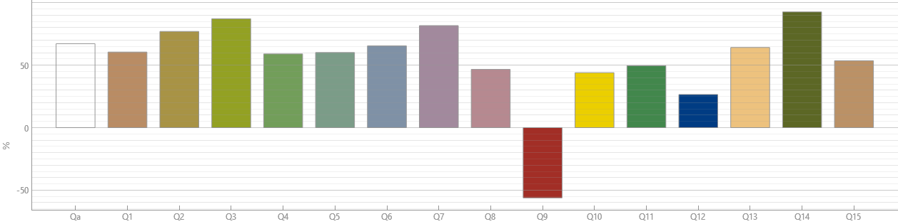
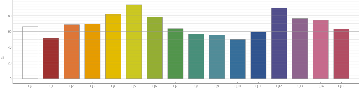
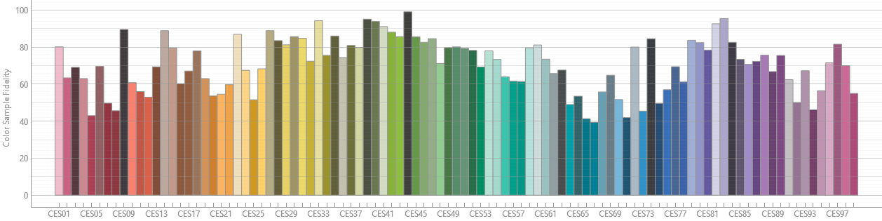
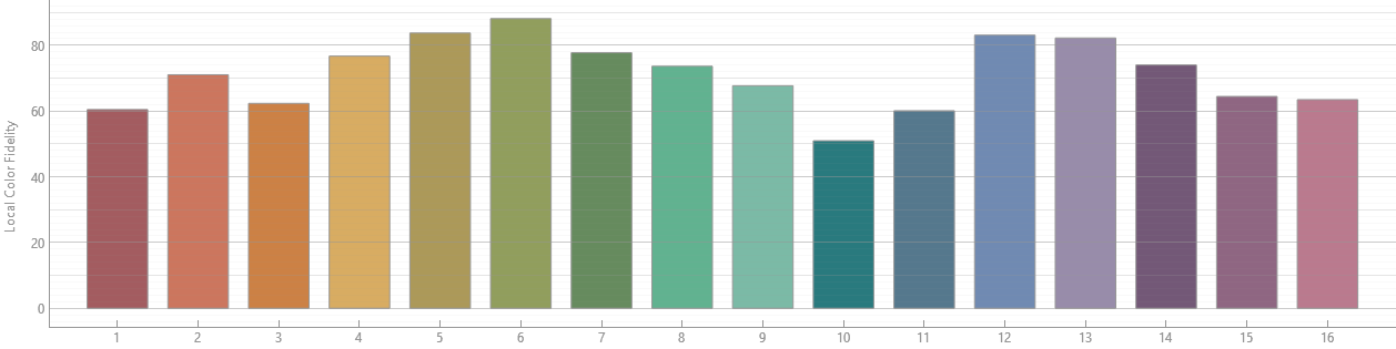
Fig. 3.10 Comparison of Color Rendering Metrics for the LED lightsource in Figure 3.7.#
See also
The (as of late) free tool BabelColor provides further radiometric analysis options.