4.5. Remote Control

This section provides a worked example on how to record and display data from spectrometers controlled by TII Spectrometry using a remote connection. The code is mean to be run in a Jupyter notebook and assumes that matplotlib is installed.

1. First, we need to import the required libraries.

   import asyncio
   import struct
   import json
   import matplotlib.pyplot as plt
   

   The last line (importing matplotlib) is optional and only required for display.

2. Next, we connect to the TII Spectrometry server.

   host = '192.168.2.180'
   port = 4711
   
   reader, writer = await asyncio.open_connection(host, port)
   print(f"Connected to {host}:{port}")
   

   Here, host is the IP-address of the machine running the TII Spectrometry spectrometer server, which is indicated in the server dialog window (Figure 2.10). port is the port of the server, 4711 by default.

3. We define a helper function to fetch data:

   async def fetch_data(writer, reader, command):
       command = command + "\n"
       writer.write(command.encode())
       await writer.drain()
       print(f"Sent: {command}. Waiting for data...")
   
       # 3. Read the 4-byte Big-Endian Length Header
       header = await reader.readexactly(4)
       msg_len = struct.unpack('>I', header)[0]
       print(f"Header received. Expecting {msg_len} bytes of JSON data.")
   
       # 4. Read the JSON payload
       payload = await reader.readexactly(msg_len)
       data = json.loads(payload.decode('utf-8'))
   
       print("Data received successfully!")
       return data
   

   This will:

   • send the command

   • read the first four bytes of the server’s response to determine the length of the JSON payload

   • read the JSON payload using the provided length

   • decode the payload into a Python dictionary

4. We can use this helper function to record spectra:

   spectrum = await fetch_data(writer, reader, "ACQUIRE")
   

   The spectrum data can be accessed using the keys documented in Section 2.1.9.1.2. For example, executing

   spectrum['timestamp']
   

   in the notebook will print the timestamp.

   '2026-03-02T17:15:18.376000+09:00'
   

5. Spectral data can be accessed using the spectrum_x and spectrum_y keys. To plot a spectrum using matplotlib, use:

   plt.plot(spectrum['spectrum_x'], spectrum['spectrum_y'])
   plt.show()
   

   

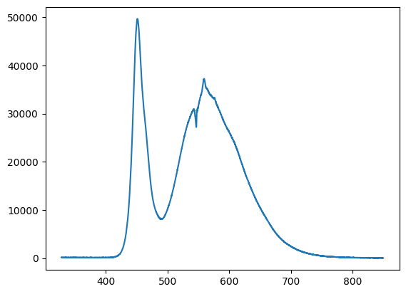
   Fig. 4.17 Plotting a spectrum using matplotlib.

6. To get the current spectrometer configuration, use the GET_CONFIGURATION command. This returns a dictionary or, in the case of multiple connected spectrometers, a list of dictionaries.

   {
       'n_average': 1,
       'spectral_domain': 1,
       'identifier': 'DS-InGaAs-256 #16052512',
       'intensity_calibration': None,
       'use_intensity_calibration': False,
       'intensity_calibration_unit': '',
       'use_nlir': False,
       'use_nlir_crop': True,
       'exposure_time': 100,
       'x_timing': 3,
       'manufacturer': 'StellarNet',
       'is_active': True,
       'use_stitching': False,
       'switchover_wl': 0
   }
   

7. To send data, we again define a helper function

   async def send_data(writer, reader, command, payload):
       command = command + "\n"
       writer.write(command.encode())
   
       payload = json.dumps(payload).encode('utf-8')
       header = struct.pack('>I', len(payload))
       
       writer.write(header)
       writer.write(payload)
       await writer.drain()
   

   This functions accepts a command and a payload in the form of a Python dictionary or list of dictionaries, encodes them into JSON, and transmits this as length-prefixed JSON data.

8. We can use this function to configure the spectrometer

   await send_data(writer, reader, "SET_CONFIGURATION", {"n_average": 1, 'exposure_time':50})
   

   Here, we set the exposure time (exposure_time) to 50 ms and the number of spectra to average (n_average) to 1.

   Multiple spectrometers can be controlled using a list:

   await send_data(writer, reader, "SET_CONFIGURATION", [{"identifier": "DS-InGaAs-256 #16052512", "n_average": 1, 'exposure_time': 100, "is_active": True}])    
   

   The identifier key is required.

9. This allows full programatic control over the spectrometer, e.g. in a loop:

   exposureTimes = [5,10,25,50,100,250,500,1000]
   
   for t in exposureTimes:
       await send_data(writer, reader, "SET_CONFIGURATION", {'exposure_time':t})
       sp = await fetch_data(writer, reader, "ACQUIRE")
       plt.plot(sp['spectrum_x'], sp['spectrum_y'], label=f"Exposure: {t} ms")
       await asyncio.sleep(1)
   
   plt.legend()
   plt.show()
   

   This snippet acquires spectra at different exposure times and plots them in a simple graph.

   

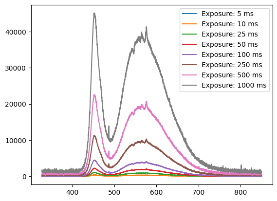
   Fig. 4.18 Plotting spectra using matplotlib.

10. When finished, it is good practice to close the connection

    writer.close()