
3.1. Time-Lapse Analysis#
Time-lapse analysis allows the visualization of the evolution of spectral parameters vs time. Available parameters are:
Sum: a running sum of the selected spectral region \(I = \sum_{x_0}^{x_1} I_x\)
Integral: the area under the curve of the selected region (computed by trapezoidal integration) \(I = \int_{x_0}^{x_1} I_x dx\). The difference to the Sum parameter is that the integral accounts for the (potentially non-constant) spacing of the data points.
Integral - BG: The area under the curve of the selected region after subtraction of the baseline. The baseline is computed as the line connecting the borders \(\rm{x}_0\) and \(\rm{x}_1\) of the selected region.
Height: The difference between the minimum and maximum intensity of the selected region.
Max. Location: The location (in units of wavelengths / wavenumber) of the point with the highest intensity.
Centroid: computes the centroid (center of mass) of the peak in the selected spectral region. For symmetric peaks, this is equal to the peak’s location, i.e. its highest value. Unlike Max. Location, Centroid can interpolate the location and thus compute peak positions at a resolution higher than the spectral resolution of the data. The center of mass is defined as: \(x_{\rm{COM}} = \frac{\sum{x_iI_i}}{\sum{I_i}}\).
FWHM: The full width at half maximum of the selected region.
Ratio: The integrated intensity ratio of two selected regions (blue and green regions in Figure 3.1)
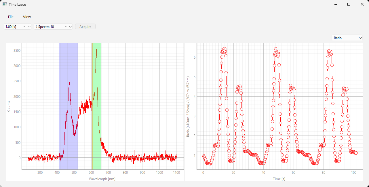
Fig. 3.1 Peak ratio analysis#
Ratio - BG: The integrated intensity ratio of two selected regions after subtracting the baseline.
Load Model: Loads a pre-trained regression model and uses this model to extract a numerical value (e.g. a concentration based on a calibration curve) from the spectra (Figure 3.2). Several models can be loaded. Models appear in the menu using their file name.
Model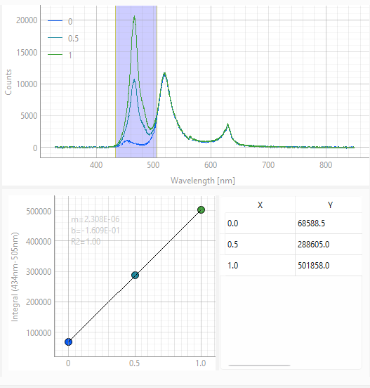 Prediction
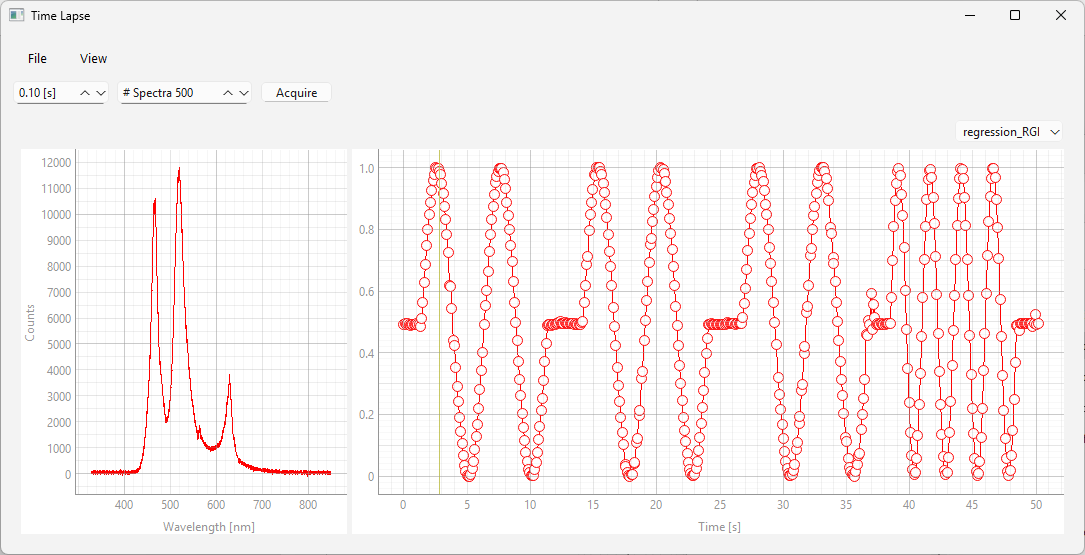
Fig. 3.2 Timelapse regression analysis#
Hint
Time traces can be exported by right-clicking on the (right) time trace view and selecting to show the Export dialogue.
3.1.1. The Time-Lapse Analysis Window#
The time-lapse analysis window can be accessed via in the time-lapse window. The analysis window has three panes:
the spectral image view (Figure 3.1). This view shows the acquired spectra as a spectral image, with the spectral dimension as the horizontal axis, the elapsed time as the vertical axis, and the spectral intensity as the image color.
the current spectrum (shown at the bottom) can be selected by dragging the vertical marker.
the spectral region of interest can be selected by moving and resizing the vertical rectangle.
the image color can be adjusted by dragging the markers in the top color scale
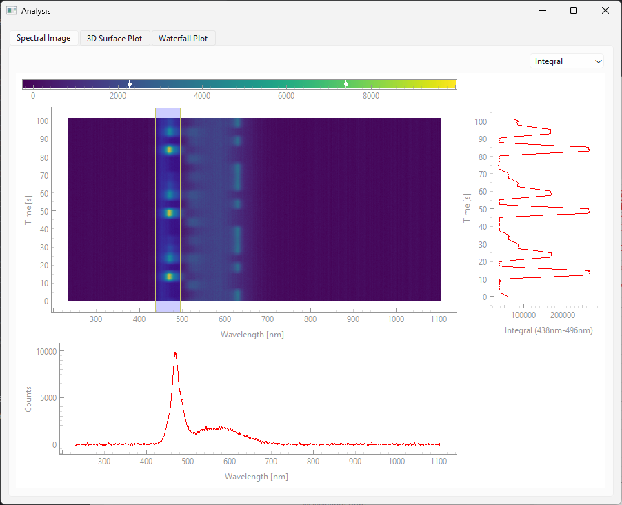
Fig. 3.3 Time-lapse Analysis - Spectral Image#
The vertical graph on the left displays a time trace of the selected parameter, similar to the time lapse window.
the surface plot view (Figure 3.4). This shows a 3D representation of the time-lapse dataset that can be rotated and zoomed using the mouse.
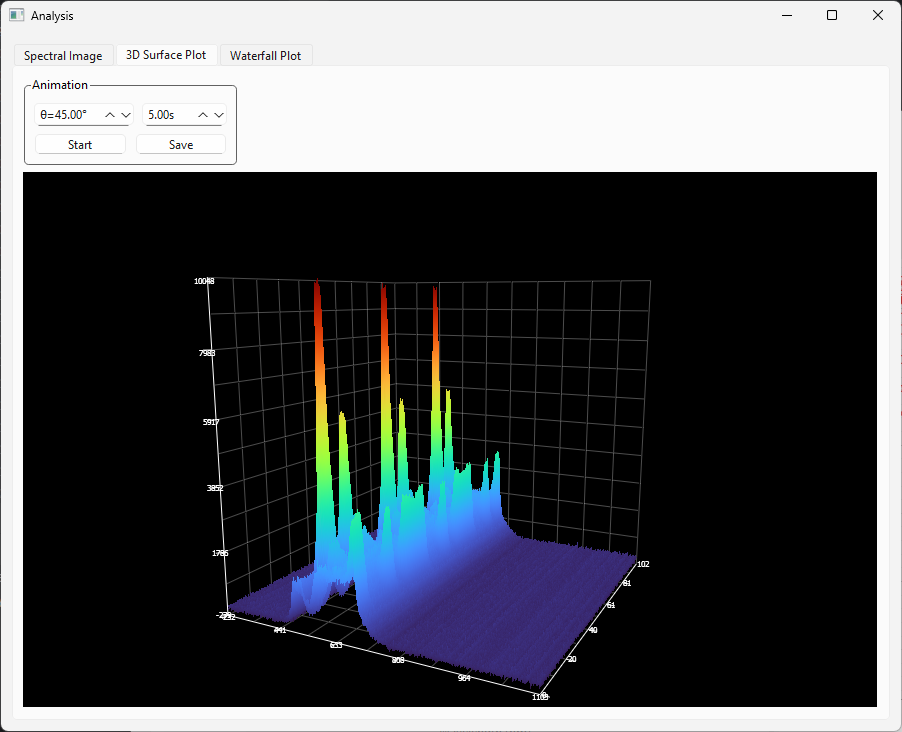
Fig. 3.4 Time-lapse Analysis - 3D surface#
the waterfall plot view (Figure 3.5). This plot is more suitable for sparse time-lapse recordings with only few acquired spectra. The (optional) coloring indicates time (in contrast to the 3D surface plot where it represents intensity).
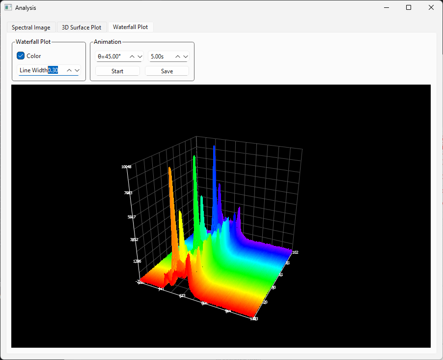
Fig. 3.5 Time-lapse Analysis - Waterfall#
Hint
The 3D surface and waterfall plots can be animated using the Animation settings box. Animations can be exported as .gif or .png using the Save button.