
2.1. General Use#
This section describes how to acquire single spectra using TII Spectrometry.
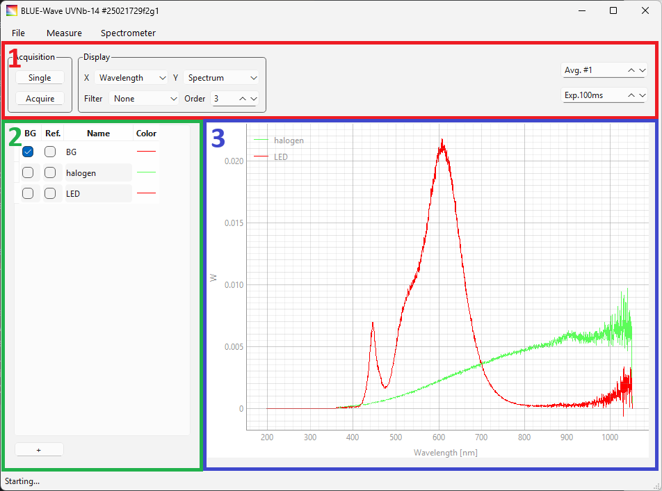
Fig. 2.1 The TII Spectrometry user interface.#
The main window of TII Spectrometry is divided into three sections:
The top bar (red box in Figure 2.1) configures spectral acquisition an display
the sidebar (green box in Figure 2.1) contains saved spectra and allows selecting background and reference spectra
The spectrum view (blue box in Figure 2.1) contains one or more spectra.
2.1.1. Connection#
To connect to a spectrometer, use any of the following methods:
select . This will connect to the first detected spectrometer.
select to open the Device Manager and select the desired spectrometer(s) from the list. For details see the section Using Multiple Spectrometers.
open a device configuration file using . This will connect to the spectrometers in the configuration file if they are connected to the computer.
If the connection was successful, the connected spectrometer(s) will be displayed in the title bar of the TII Spectrometry window and the Single and Acquire buttons become active (Figure 2.1).
2.1.2. Device Configuration#
The top bar of the TII Spectrometry window (red box in Figure 2.1) allows the configuration of the most relevant experimental parameters:
2.1.2.1. Spectral Acquisition#
- Single
Acquires a single spectrum using the current configuration
- Acquire
Starts the spectrometer and continuously acquires spectra. Clicking the Stop button stops continuous acquisition.
- Avg. #
Selects the number of spectra to average. Use this to improve the signal-to-noise ratio
- Exposure Time
The exposure time of the detector in milli-seconds.
See also
Averaging and exposure time can be set individually for each connected spectrometer, see section Using Multiple Spectrometers for details.
2.1.2.2. Display#
This section allows to change how spectra are displayed in the spectrum view (blue box in Figure 2.1).
- X
Selects the spectral domain:
wavelength in nm
wavenumber in 1/cm
- Y
Selects what parameter to display on the vertical axis:
Spectrum displays the spectrometer counts. If a background spectrum has been recorded, it is subtracted before display.
Absorbance computes an absorbance spectrum \(A = -\log_{10} \frac{I}{I_0}\), where \(\rm{I_0}\) is a reference spectrum
Transmittance computes an transmittance spectrum \(T = \frac{I}{I_0}\), where \(\rm{I_0}\) is a reference spectrum
Note
The Absorbance and Transmittance mode require a reference spectrum.
- Filter
Activates spectral post-processing to reduce noise (Figure 2.2). Available filters are:
None: No filtering, the spectrum is left untouched.
Moving Avg.: A moving average filter.
Binomial: A binomial (Gaussian) filter.
- Order
Selects the window size of the moving average of binomial filter (Figure 2.2).
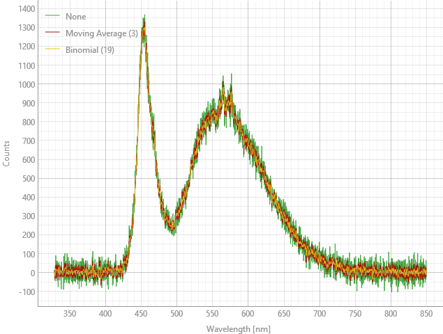
Fig. 2.2 Effect of Filter and Order.#
2.1.2.3. Device Configuration Files#
Device configuration (including multiple spectrometers) can be saved to disk using . Configuration files include:
the connected spectrometers
external triggering (if supported)
various device-dependent parameters
To load a configuration file, use . An example configuration file is displayed below.
{
    "spectrometers": [
        {
            "n_average": 1,
            "spectral_domain": 1,
            "intensity_calibration": [

            ],
            "use_intensity_calibration": false,
            "intensity_calibration_unit": "W",
            "identifier": "Aris S/N 118",
            "use_nlir": false,
            "use_nlir_crop": true,
            "exposure_time": 1.0,
            "gain": 0,
            "external_trigger": false,
            "manufacturer": "Avenir"
        }
    ]
}
Note
Background and reference spectra are not saved in the device configuration but can be saved and loaded from disk using the save dialogue and saving in the .hdf5 format.
Hint
A configuration file can be loaded upon application start by using the -c command line option, e.g. (on Windows) TII-Spectrometry.exe -c myconfig.json, where myconfig.json is the name of a config file.
2.1.3. Recording Spectra#
To record a single spectrum, click Single in the top bar. To continuously acquire spectra, click Acquire, to stop spectral acquisition, click Stop.
Warning
Spectra will not be saved during continuous acquisition. To acquire spectra continously at regular time intervals, use a time-lapse acquisition.
2.1.4. Saving Spectra#
To save the currently displayed spectrum, click the + button at the bottom of the sidebar. This will add the spectrum to the sidebar. In the sidebar, you can:
select several spectra (using Ctrl+Click or Shift+Click) to display in the spectrum view, e.g. for comparison
change the name of a spectrum by double-clicking on the spectrum’s name
change the spectrum’s color by double-clicking on the color
delete spectra by
pressing the Delete key
right-clicking on the selected spectra and selecting from the context menu
reorder spectra using drag&drop
copy the selected spectra’s data to the system clipboard in the
.csvformat using or Control-Cduplicate spectra by selecting from the context menu
reprocess spectra selecting from the context menu
Note
Saved spectra are immutable. To change a spectrum, e.g. using filtering, background subtraction or by changing its spectral domain, select from the context menu. To perform reprocessing on a copy (to leave the original spectrum untouched), select followed by .
To save the selected spectra, select from the context menu. See the section File Input & Output for details. To select all spectra, use Control-A.
Hint
If more than two spectra are selected, the option will become available. This allows applying a color scale to differentiate the selected spectra, which can be useful to highlight spectral differences of spectra acquired under different conditions (Figure 2.3)
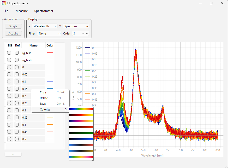
Fig. 2.3 Colorizing Traces#
2.1.4.1. Background & Reference Spectra#
to select a saved spectrum as the background spectrum, check the BG column in the spectra sidebar. The intensity values of the background spectrum will be subtracted from all subsequent recorded spectra.
to select a saved spectrum as the reference spectrum, check the Ref. column in the spectra sidebar. This will enable Absorbance and Transmittance calculations.
Tip
Meaningful background and reference spectra have to be acquired under experimental conditions similar to the acquat spectral recordings, e.g. using the same exposure time and illumination. To improve the signal-to-noise ratio of background or reference spectra for subsequent calculations:
2.1.5. Spectrum Display#
The spectrum view (blue box in Figure 2.1) displays one or more selected spectra. The view can be adjusted
using the scroll wheel to zoom
dragging while holding down the right mouse button to zoom
dragging while holding down the left mouse button to pan
To reset the display (autoscaling all traces)< click the A button at the bottom left corner.
Additionally, the context menu (right-click) offers the following options:
: autoscales the view
and adjust the visible X and Y range ad allow autoscaling one axis only
. Displays a cursor or region-of-interest selector
the Cursor () is a vertical bar that can be dragged using the mouse. The position of the cursor (x value) and the spectral intensity at the selected position (y value) are displayed at the bottom of the TII Spectrometry window (Figure 2.4).
the region-of-interest (ROI) selector () marks a region that can be dragged and resized using the mouse. Various parameters of the selected region are displayed at the bottom of the TII Spectrometry window (Figure 2.4). For details on how the parameters are computed, see Section 3.1.
Cursor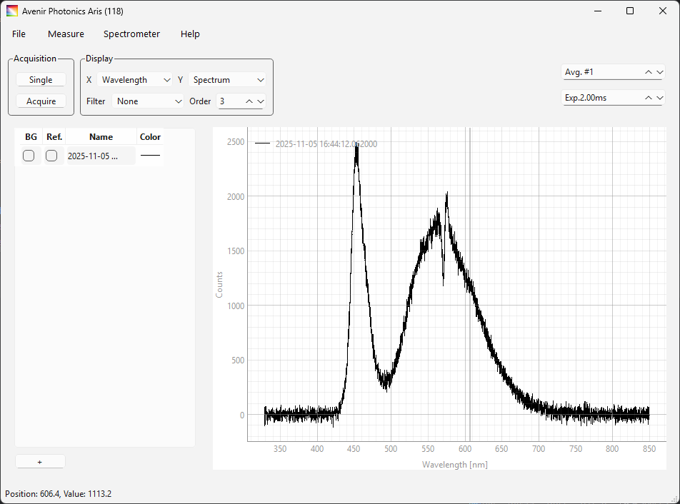 ROI
ROI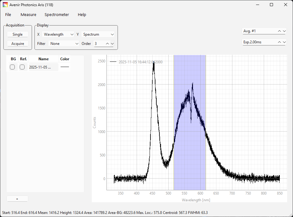
Fig. 2.4 Spectrum View - Cursor Display#
toggles peak position display in the spectrum view (Figure 2.5)
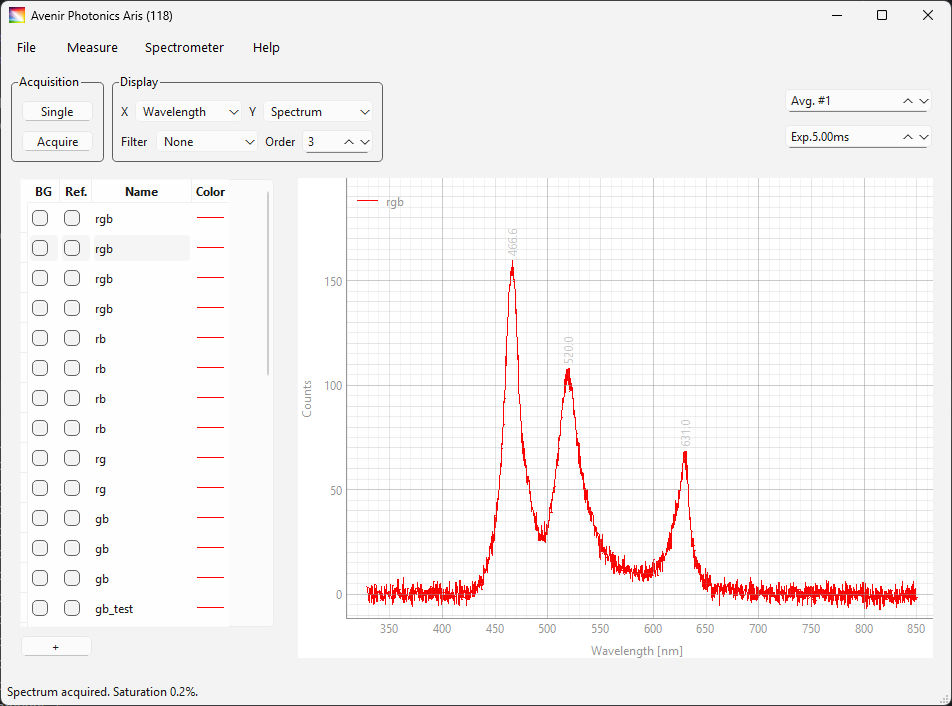
Fig. 2.5 Peak Display#
displays the Acquisition Parameters window (Figure 2.6), which contains metadata of the acquired spectrum.
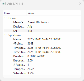
Fig. 2.6 The Acquisition Parameters Window.#
displays the Export Dialog window (Figure 2.7). This window allows:
the export of the plot as an image
the export of the plot’s underlying data as
.csvor.hdf5
to disk or the system clipboard.
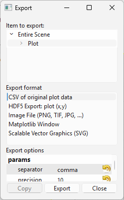
Fig. 2.7 The Export Dialogue Window#
Hint
The spectrum view graph can also be copied to the system clipboard using standard system commands (e.g. Control-C on Windows).
Important
The
.hdf5files exported using the Export Dialogue cannot be re-imported into TII Spectrometry. For round-tripping, use the command in the spectrum sidebar.
2.1.6. Intensity Calibration#
Intensity calibration describes the process of using a spectrum of a reference light source with a a known intensity distribution (typically a black-body emitter with a well-characterized color temperature) to correct the sensitivity and throughput of the spectrometer and input optics at different wavelengths. If the radiance or irradiance of the light source are known, recorded spectra can, in addition, be made fully quantitative, which is essential for many applications of radiometry.
TII Spectrometry offers two options for calibration:
direct calibration using a well-characterized light source
indirect calibration using sensitivity data supplied by the manufacturer data that contains the spectrometer sensitivity at a given wavelength.
2.1.6.1. Direct Calibration#
To calibrate a spectrometer:
record a spectrum of the reference light source (using appropriate acquisition settings and, if required, background subtraction)
Important
Since the calibration curve will be calculated by division using the intensity of the reference lightsource and the reference spectrum, a high signal-to-noise ratio of the calibration spectrum is advisable.
select to display the calibration window (Figure 2.8)
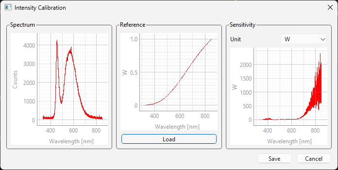
Fig. 2.8 The Calibration Window#
The spectrum of the reference light source is displayed in the left-most graph. To load the reference intensity data, click the Load button and select the reference data
Important
reference data is expected to be in a two-column
.csvformat (Listing 2.1) with no header.193.00 0.0000E+000 193.50 0.0000E+000 194.00 0.0000E+000
Here,
the first column contains the wavelength in nanometers or wavenumber in 1/cm
the second column contains the reference value of the light source, e.g. spectral power in W.
the spectral range of the reference data is expected to match (or exceed) the spectral range of the recorded reference spectrum. This means that the spectral domain (wavelength or wavenumber) has to match as well
the reference data will be interpolated to match the sampled wavelengths of the recorded spectrum
The reference intensity data will be displayed in the center graph.
Select the unit of the reference intensity
The calibration curve (sensitivity curve) will be displayed in the right-most graph
Click Save to accept the calibration.
Note
The sensitivity curve is normalized by the exposure time. This means the exposure time can be varied during subsequent spectral acquisitions to achieve the desired signal-to-noise ratio or to avoid saturating the detector…
To use the intensity calibration, check . The intensity calibration will be applied to subsequently recorded spectra.
Hint
Calibration data can be saved in a device configuration file so this procedure only has to be reperformed if the optical setup changes.
See also
See the appliction example The Solar Spectrum for additional hints and information.
2.1.6.2. Indirect Calibration#
To load sensitivity data:
Open the calibration window (Figure 2.8)
Click Load and select the calibration data file.
Click Save to apply the calibration data.
For indirect calibration, a spectrum of a well-characterized light source is not required. Calibration data will be saved along with the device configuration.
Important
Currently supported sensitivity files are .cal files supplied by StellarNet.
2.1.7. Wavelength Calibration#
Whereas intensity calibration describes the calibration of the vertical (intensity) axis of a spectrum, wavelength calibration affects the horizontal (wavelength or wavenumber) axis. Wavelength calibration can be performed using to display the wavelength calibration window (Figure 2.9).
Important
Wavelength calibration requires a line emission light source with known spectral characteristics, e.g. a mercury, mercury-argon, or neon lamp.
Hint
Small, portable spectrometers with fixed grating generally don’t require frequent recalibration. In addition to calibration, the functionality provided by the wavelength calibration window is also useful to verify spectrometer wavelengths.
Note
Wavelength calibration is only applicable to grating-based spectrometers. Interferometry-based FTIR spectrometers cannot be calibrated in this manner.
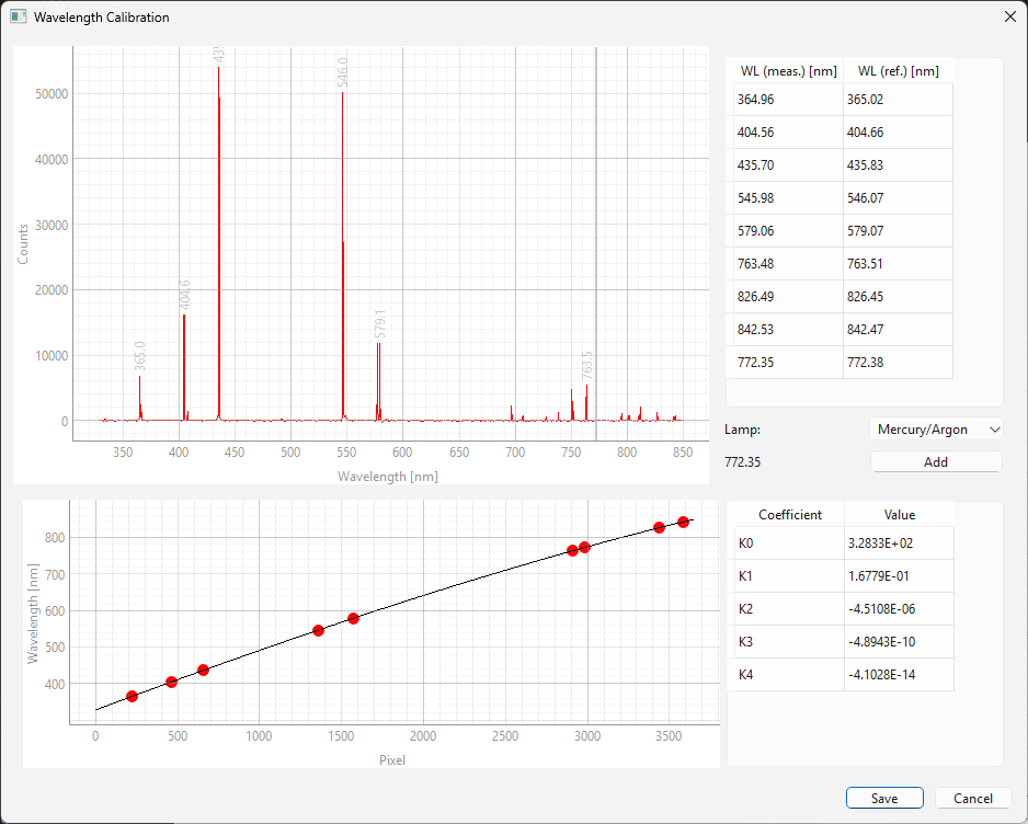
Fig. 2.9 The Wavelength Calibration Window#
To perform a wavelength calibration / verification:
Record a spectrum of a well-characterized calibration light source with known spectral emission lines.
Important
To accurately determine peak positions, it is critical not to saturate the detector.
Open the wavelength calibration window via {menuselection}Spectrometer –> Wavelength Calibration (Figure 2.9). In this window:
Top-left graph: Displays the recorded calibration spectrum.
Top-right table: Lists the measured pixel/wavelength positions of detected peaks alongside their known reference wavelengths.
Bottom-left graph: Displays the calibration curve mapping detector pixels to reference wavelengths. This mapping uses a 4th -degree polynomial fit (indicated by the black line).
Bottom-right table: Displays the resulting calibration coefficients.
Peaks are automatically detected in the recorded spectrum; these are listed in the table and indicated in the graph. For each detected peak, a reference wavelength must be assigned. This can be done by:
by entering the known values directly into the top-right table.
by selecting the type of calibration lamp used in the Lamp drop-down menu. TII Spectrometry will try to automatically assign the detected peaks to the known wavelengths of the calibration light source
Note
Currently, TII Spectrometry supports mercury-argon (Hg-Ar) lamps.
The bottom left graph will update automatically as reference wavelengths are assigned.
To manually manage peaks,
To add a peak: Drag the cursor in the top left graph to the desired position position and click the Add button. The currently selected wavelength (cursor position) is displayed next to the Add button.
To add a row: Select from the context menu in the top-right table or us the Tab key in the right-most cell of the last row to add a new entry. Then enter the measured and reference wavelengths.
To delete a peak: Use the Delete key or select from the context menu.
Important
For a high-quality fit, it is crucial that the selected peaks cover the full spectral range of the detector. Manually adding peaks near the detector edges is highly recommended.
The fit and coefficients update in real-time. Click Save to apply the new calibration. To discard changes and revert to the factory calibration, click Cancel.
Note
Calibration coefficients may also be entered manually in the bottom-right coefficients table.
Calibration values will be saved in the device configuration file and the new calibration will be applied to subsequently recorded spectra.
2.1.8. File Input & Output#
Spectral data can be exported from TII Spectrometry in a variety of ways:
selecting one or more spectra in the spectrum sidebar and selecting from the context menu (or using the shortcut Control-C) copies the spectral data to the system clipboard using the
.csvformat. This allows direct pasting into third-party graphing or analysis software.selecting one or more spectra in the spectrum sidebar and selecting from the context menu (or using the shortcut Control-S) displays a file dialogue and allows saving the spectral data to disk. Available formats are
.csvand.hdf5..csvfiles enjoy widespread support and can be imported by virtually all third-party software.hdf5files are the native file format of TII Spectrometry and can be re-imported for later analysis. These files can be read using a wide variety of applications including MATLAB, Igor Pro, and Origin Pro. Python support is available via the h5py package. In addition to the wavelength and intensity data, this format also containsraw intensity values (before background subtraction etc.)
timestamps
additional metadata
Tip
A convenient way to inspect
.hdf5files is the https://myhdf5.hdfgroup.org/ website.
using the Export Dialogue in the spectrum view.
Note
The recommended output format is .hdf5 exported from the spectrum sidebar, which retains most information.
To re-import .hdf5 data into TII Spectrometry,
use and select a
.hdf5file from the file dialoguedrag and drop one or more
.hdf5files onto the spectral sidebar
2.1.9. Remote Control#
TII Spectrometry exposes a TCP/IP server and a HTML webserver that can be used to control and monitor the connected spectrometer(s) remotely. This functionality can be accessed via to display the remote control dialog window (Figure 2.10).
2.1.9.1. TCP/IP Server#
The TCP/IP server can be accessed from the TCP/IP tab (Figure 2.10).
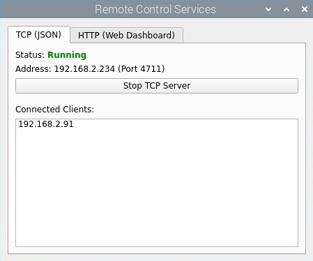
Fig. 2.10 The TCP/IP Remote Control Server Dialog Window#
Note
The TCP/IP server functionality of TII Spectrometry is designed to:
work in tandem with configuration files to provide remote access to a single spectrometer (or set of spectrometers) for routine analysis. As the server configuration is saved to the configuration file, starting TII Spectrometry using the
-ccommand line option willconnect to the configured spectrometers,
apply the configuration (exposure time, calibration, etc.),
start the server
This allows convenient remote control using a headless machine as the server.
provide the ability to use a variety of spectrometers via TII Spectrometry from user-defined scripts using a common interface, see the application example Remote Control for details.
allow an instance of TII Spectrometry running on a different machine to connect to and control remote spectrometers.
See also
The section Device Manager describes how to use TII Spectrometry as both client and server to control single or multiple local and/or remote spectrometers.
2.1.9.1.1. Server Configuration#
This window contains the following controls:
- Start/Stop Button
Starts or stops the server. The server status is indicated in the status label.
- Connect to
Displays the IP address of the server. Use this to connect to the server.
Important
The ability to connect to an IP address depends on the network layout. Connections work most reliably if the server and client machines are part of the same subnet.
- Connected Clients List
Shows a list of connected client machines
Hint
The server accepts connections on port 4711 by default. This can be changed in the configuration file.
To use the server, simply click the Start Server button. The server will wait for client connections and deliver spectra (using the current configuration) on request.
2.1.9.1.2. Client Configuration#
The TII Spectrometry server accepts the following commands:
Important
Commands should be terminated with a newline character (\n).
ACQUIREStarts a single spectral acquisition with the currently configured parameters.
The returned data is provided as length-prefixed JSON data:
the first four bytes contain the length of the data as a Big-Endian unsigned integer
the remaining data is the JSON payload as a UTF-8 encoded string with the following data fields:
timestamp: contains the time stamp of the spectrum in ISO 8601 formatspectrum_x: contains the x-values (wavelength or wavenumber) of the spectrum as a list of floating-point numbersspectrum_y: contains the y-values (intensity, absorbance, etc.) of the spectrum as a list of floating-point numbersspectrometer: contains the name of the spectrometerdomain: contains the spectral domain (wavenumber of wavelength)mode: indicates what parameter is displayed on the vertical axis (absorbance, intensity, etc.)
{
    "timestamp": "2026-03-02T16:55:38.026000+09:00",
    "spectrum_x": [328.3851318359375,
                   328.55224609375,
                   328.7193603515625],
    "spectrum_y": [41.23124694824219,
                   46.98746871948242,
                   35.47492980957031],
    "spectrometer": "Aris S/N 118",
    "domain": "WAVELENGTH",
    "mode": "SPECTRUM"
}
GET_CONFIGURATIONReturns the configuration of the currently connected spectrometer(s) as a JSON object.Valid keys vary by device. The format follows the format of the configuration file.
SET_CONFIGURATIONApplies a new configuration to the connected devices.
the new configuration should be provided as a length-prefixed JSON object
for single spectrometers, the JSON data should be a dictionary
for multiple connected spectrometers, JSON data should be a list of dictionaries. The
identifierkey is required to control which spectrometer the new parameter set should be applied to.
Tip
Top avoid unneccessary hardware reconfiguration, specify only parameters that should be changed in the JSON data
See also
See the application example Remote Control for an example how to connect to the TII Spectrometry server using Python.
2.1.9.2. HTML Webserver#
The HTML server can be accessed from the HTML tab (Figure 2.11).
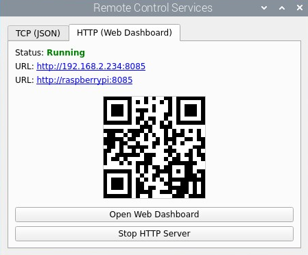
Fig. 2.11 The HTML Webserver Dialog Window#
- Status
Displays the status of the server - either running or stopped
- URL
Displays the address of the server in the form
ip_address:portandhost_name:port.- QR Code
Displays the server address encoded as a QR code.
- Open Web Dashboard
Opens the server dashboard in the local browser
- Start / Stop
Starts or stops the server
Tip
Since network access is relatively slow, spectral acqusition is throttled.
2.1.9.2.1. Web Dashboard#
The HTML Dashboard (Figure 2.12) is a modern, responsive web application (Figure 2.14) that mirrors the control options available in TII Spectrometry.
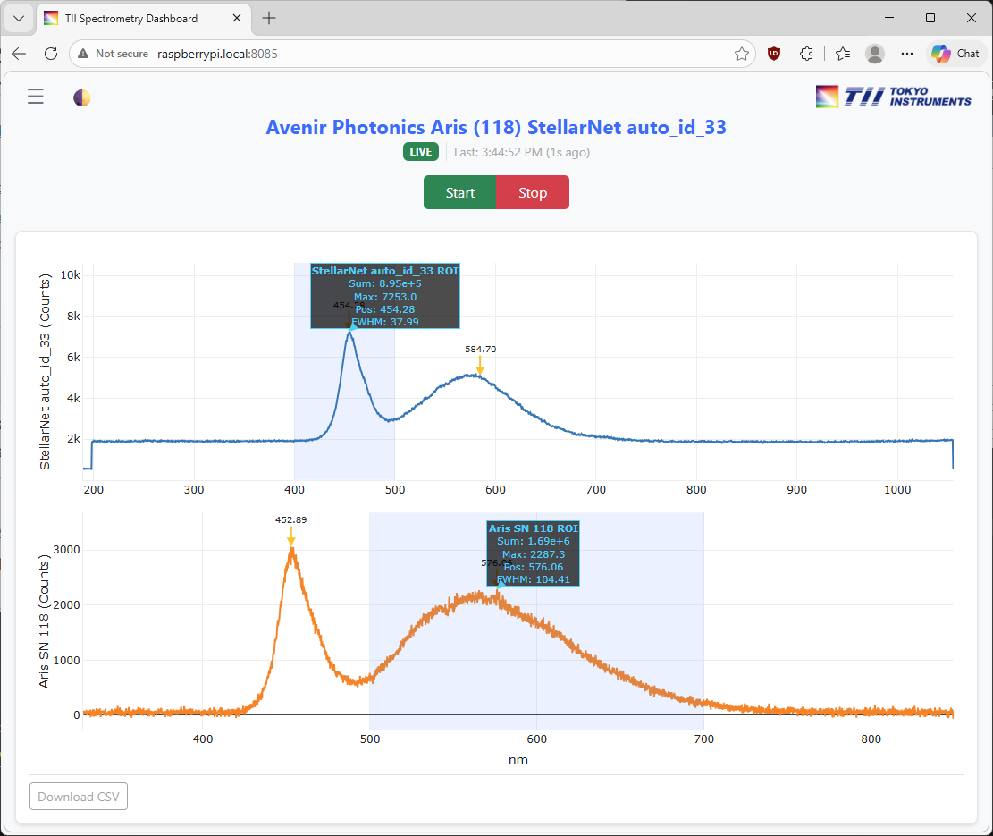
Fig. 2.12 The HTML Dashboard#
Features include:
control of multiple spectrometers
controlling exposure time and averaging
selecting x and y-axis units of the displayed spectra
recording background and reference spectra
adjusting the displayed region in the graphs
computation of spectral metrics (running sum, maxmimum value, maximum location, FWHM) for a selected region
export as image or
.csvdata
Most of these controll options are available in the sidebar (Figure 2.13), which can be accessed using the ☰ button.
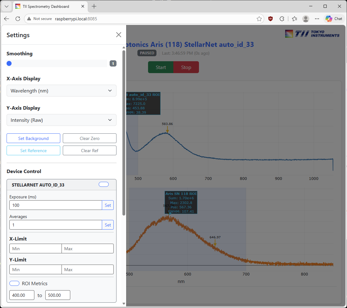
Fig. 2.13 The HTML Dashboard Sidebar#
The Start button starts the spectrometer, the Stop button pauses spectral display.
Important
While the web dashboard gives access to a wide range of configuration options, it is important to keep in mind that the spectrometer is a shared resource. If multiple clients are connected, each connected client can change acquisition parameters for all other clients. The only exception is the Stop button, which will not stop the spectrometer but only pause client updates. The spectrometer server will stop the devices if no clients make requests for new spectra. Similarly, the dashboard will reflect changes made to acquisition parmeters made in the app running on the host computer.
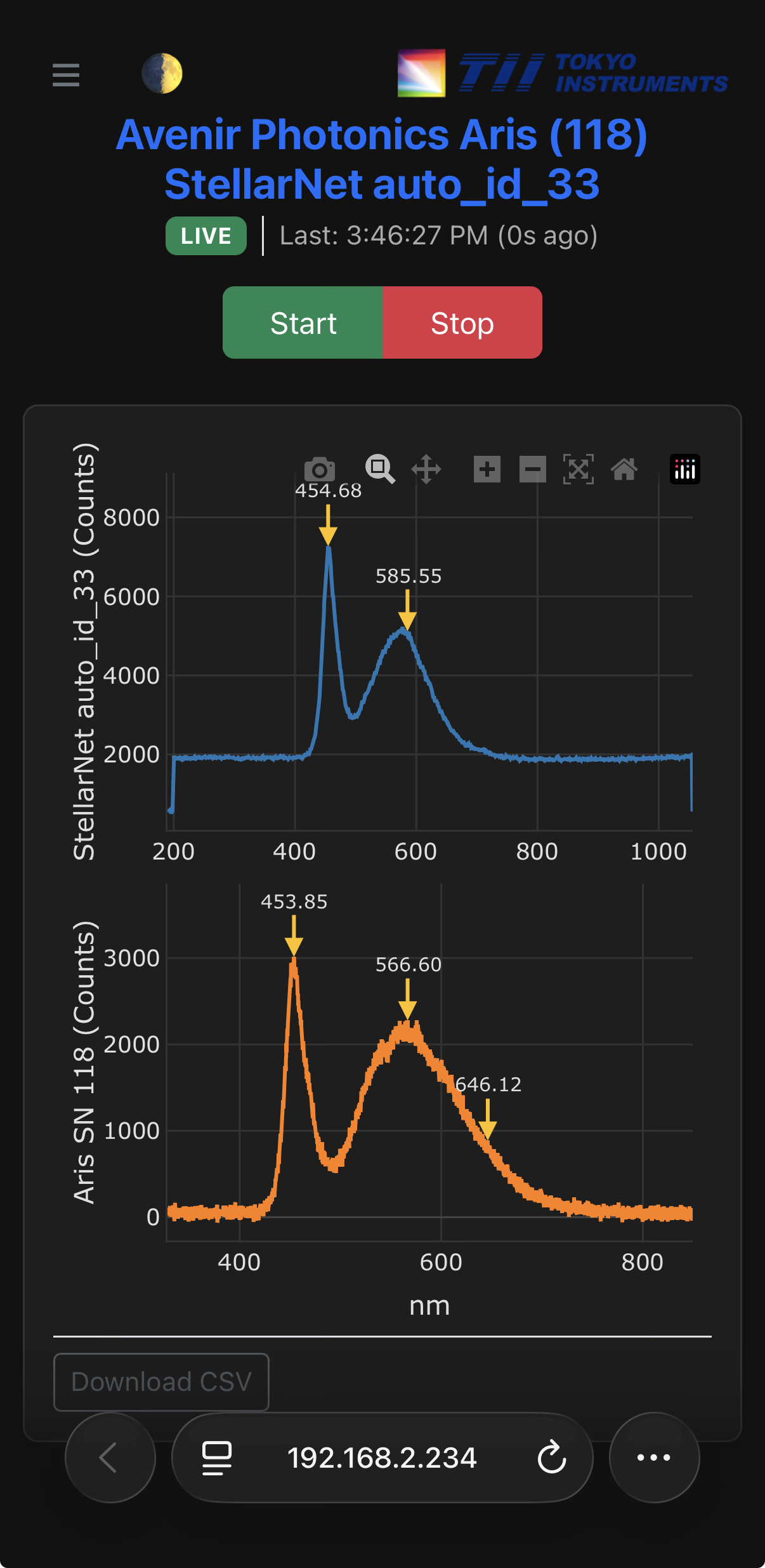
Fig. 2.14 The HTML Dashboard running on a mobile device.#