4.6. Characterization of an LED-based Solar Simulator

This application example explores the characterization and control of an LED-based solar simulator (G2V Pico). It leverages several key features of TII Spectrometry:

• Multi-spectrometer control: The solar simulator covers a spectral range from visible to near-infrared light, exceeding the capabilities of a typical single spectrometer. TII Spectrometry enables the simultaneous control of multiple devices to expand the spectral range, allowing the acquisition of the full simulated solar spectrum in a single shot.

• Intensity calibration: To acquire quantitative spectra, the sensitivity curve of the spectrometers must be accurately determined. When multiple devices are used, intensity calibration is crucial to account for varying spectral sensitivities. Stitching can then be employed to generate a continuous, seamless spectrum over a broad range.

• Remote control: TCP/IP-based remote communication is used to automate spectral acquisition and orchestrate hardware between the computer-controlled light source and the spectrometers.

In this setup, TII Spectrometry controls the hardware, performs spectral processing and intensity calibration, and delivers data ready for custom scripts for visualization, analysis, or hardware feedback loops. Beyond providing a hardware abstraction layer for devices from different manufacturers, this approach facilitates a flexible experimental workflow, allowing users to combine manual control with scripted acquisition as needed.

4.6.1. Materials & Methods

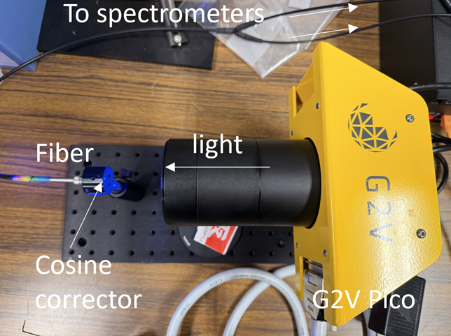
Fig. 4.19 Optical setup used to characterize the G2V Pico solar simulator.

Figure 4.19 illustrates the optical setup: The light emitted by the solar simulator is collected via a cosine corrector (diffuser) and coupled into a bifurcated optical fiber. A StellarNet BlueWave (utilizing a Silicon CCD detector for the UV-Vis-NIR range) and a DWARF-Star (utilizing an Indium Gallium Arsenide (InGaAs) photodiode array for the NIR range) are used to acquire spectra covering the range from 200 to 1750 nm. Both spectrometers were calibrated using a certified calibration lamp (Figure 4.20). The switchover point between the two spectrometers was set to 930 nm, representing an optimal crossover region where both detector types maintain high quantum efficiency and low noise, thereby minimizing stitching artifacts near the band edges.

Hint

Calibration data is saved in TII Spectrometry configuration files, meaning this procedure only needs to be performed once, provided the optical setup (fiber, diffuser, etc.) remains unchanged.

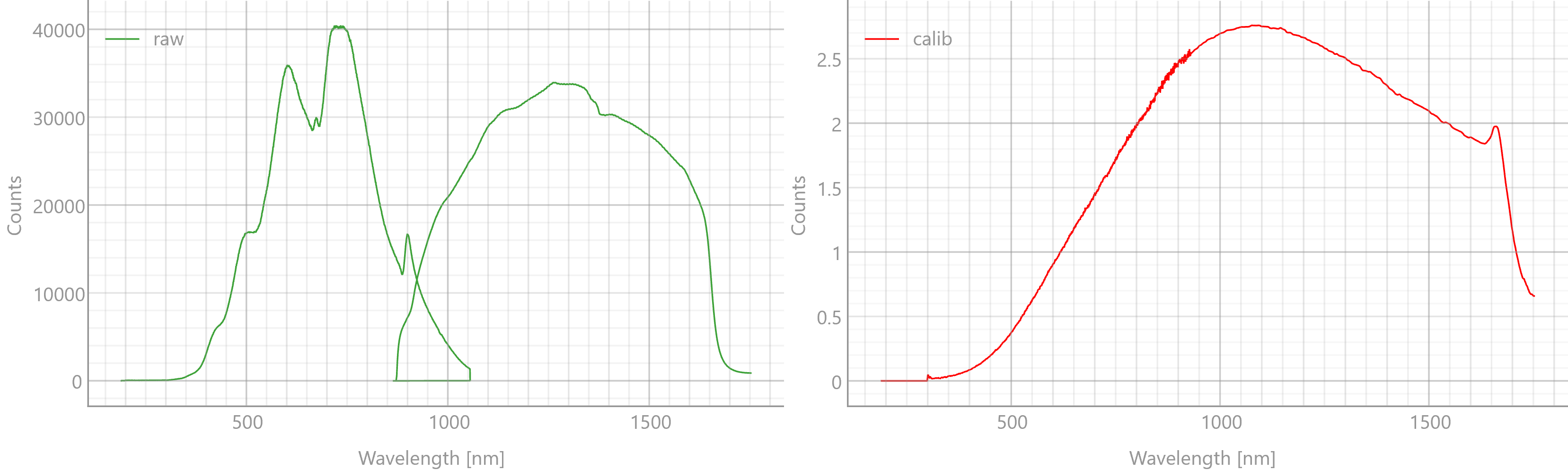
Fig. 4.20 Calibration of the dual-spectrometer setup using a calibration lamp (black body emitter with a color temperature of 2800 K): Raw data (left) and data after intensity calibration (right).

Standard spectral and atmospheric calculations were performed using pvlib (specifically implementing the SPECTRL2 clear-sky model). Stellar spectra were obtained from the Pickles catalogue via pycles. The G2V Pico solar simulator was controlled using the G2VPico library.

4.6.2. Results

4.6.2.1. Preset Spectra

The manufacturer provides spectral presets to simulate commonly used solar standards (Figure 4.21). The acquired spectra (orange traces) were compared to the ASTM G173-03 standard spectra (black) provided by pvlib.

• AM0 (Air Mass 0): The extraterrestrial solar spectrum outside the Earth’s atmosphere, which is the standard reference for testing solar cells designed for space applications (e.g., satellites).

• AM1.5G (Global): The standard spectrum for terrestrial photovoltaic testing, representing the total solar radiation (direct and diffuse) incident on a 37° tilted surface (which represents the mean latitude of the continental United States).

• AM1.5D (Direct): The direct component of the terrestrial radiation, which excludes diffuse sky radiation and is typically used to evaluate concentrating photovoltaic (CPV) systems.

As expected, the agreement between the simulated and standard spectra is excellent. Notably, the acquired spectra are continuous, with no visible artifacts at the switchover point between the two spectrometers. Furthermore, the measurements accurately reproduce both the spectral shape and the absolute irradiance, demonstrating the effectiveness of the intensity calibration.

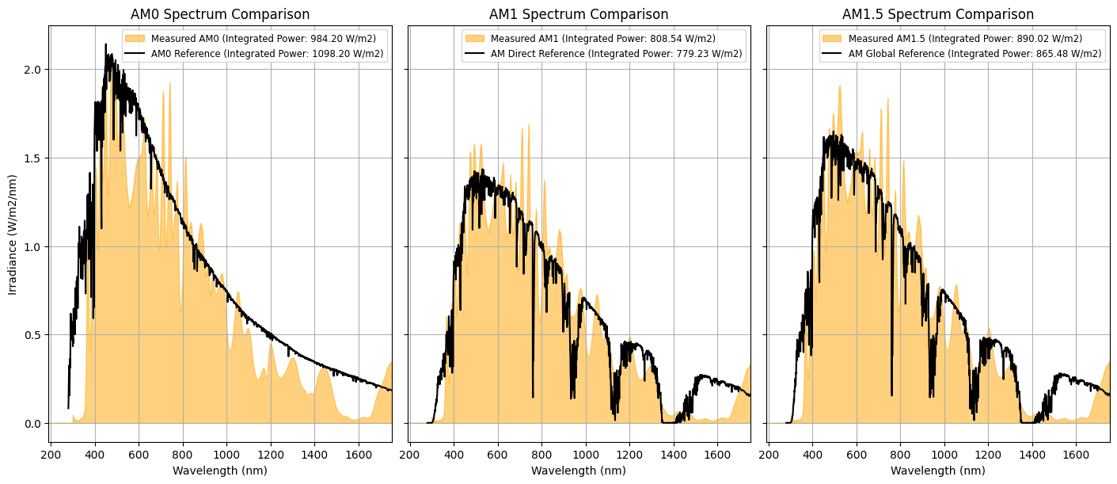
Fig. 4.21 The extraterrestrial (AM0) (left), direct (AM1.5D) (center), and global (AM1.5G) (right) solar spectra.

The IEC 60904-9 (JIS C 8912) standard defines classifications for solar simulators based on three key performance metrics: spectral match, spatial non-uniformity of irradiance, and temporal instability of irradiance. For the spectral match metric:

• The spectral match ratio \(\text{Ratio}_{\text{bin}} = \frac{\%_{\text{meas}}}{\%_{\text{ref}}}\) describes how well the integrated intensity across a specific wavelength interval (bin) matches the reference solar spectrum. In the older version of the standard, the spectral match is evaluated across six designated wavelength intervals covering the 400–1100 nm range (400–500 nm, 500–600 nm, 600–700 nm, 700–800 nm, 800–900 nm, and 900–1100 nm).

The 2020 revision of the standard (IEC 60904-9:2020) extended the evaluated range to 300–1200 nm to better match modern wide-bandgap and multi-junction PV architectures, introducing the following updates:

• The spectral match ratio is evaluated across six bins, but the bins are now defined such that each contains exactly 16.67% of the total integrated reference irradiance.

• Spectral coverage (SPC) quantifies the percentage of the integrated AM1.5G reference irradiance that is actively represented by the simulator’s output:

  \[ \text{SPC} = \left( \frac{\int_{\Lambda} E_{\text{ref}}(\lambda) \, d\lambda}{\int_{300}^{1200} E_{\text{ref}}(\lambda) \, d\lambda} \right) \times 100\% \]

  A wavelength \(\lambda\) is considered “represented” only if the simulator’s spectral irradiance (\(E_{\text{sim}}(\lambda)\)) is at least 10% of the reference spectrum’s irradiance (\(E_{\text{ref}}(\lambda)\)) at that specific point:

  \[ \Lambda = \{ \lambda \in [300, 1200] \mid E_{\text{sim}}(\lambda) \geq 0.1 \times E_{\text{ref}}(\lambda) \} \]

• Spectral deviation (SPD) measures the overall mismatch between the simulator’s emission and the reference spectrum:

  \[ \text{SPD} = \left( \frac{\int_{300}^{1200} |E_{\text{sim}}(\lambda) - E_{\text{ref}}(\lambda)| \, d\lambda}{\int_{300}^{1200} E_{\text{ref}}(\lambda) \, d\lambda} \right) \times 100\% \]

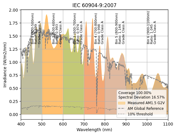
Fig. 4.22 Spectral match ratio of the G2V Pico across the 400–1100 nm range.

Figure 4.22 shows the results for the AM1.5G spectrum obtained from the G2V Pico evaluated across the 400–1100 nm range. The spectral match ratio for each of the six bins falls entirely within the 0.75 to 1.25 range (within 25% deviation from the reference), making this a Class A device for spectral match. The spectral coverage (calculated for the same wavelength range) is 100%, and the spectral deviation is 16.6%. These values are in line with the manufacturer’s nominal specifications.

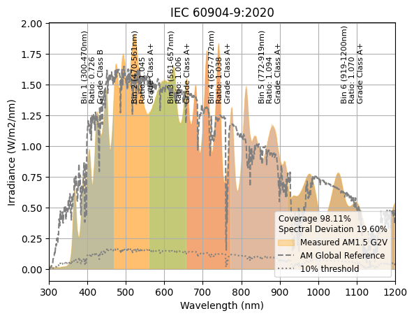
Fig. 4.23 Spectral match ratio of the G2V Pico across the 300–1200 nm range.

Figure 4.23 contains the characterization according to the newer IEC 60904-9:2020 standard. Because the Pico’s light emission only starts at approximately 350 nm, the spectral match ratio for the first bin (300–470 nm) falls outside the Class A limit and drops to Class B. However, all other bins comfortably match the tighter Class A+ standard. Due to the lack of near-UV emission in the 300–350 nm range, the overall spectral coverage also drops, and the spectral deviation increases to 19.6%.

The JIS C 8904-9 standard includes additional specifications for specialized photovoltaic technologies:

• Stacked, multi-junction solar cells (such as GaInP/GaAs/Ge tandem cells): For evaluating these devices, narrower 50 nm wavelength bins are employed, as multi-junction solar cells typically exhibit sharp quantum efficiency cutoffs at their sub-cell interfaces.

• Thin-film solar cells based on Copper Indium Selenide (CIS) or Copper Indium Gallium Selenide (CIGS): Unlike standard crystalline silicon cells, which lose sensitivity rapidly beyond 1100 nm due to the bandgap limit of Silicon, CIS/CIGS thin films can absorb light much deeper into the near-infrared (NIR) spectrum—extending all the way to 1300 nm. Consequently, the standard defines specific bins up to 1300 nm for these technologies.

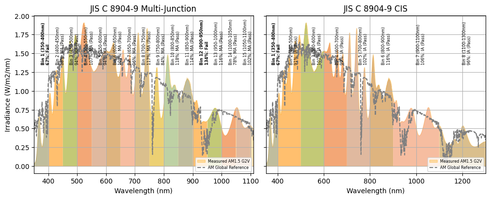
Fig. 4.24 Spectral match ratio of the G2V Pico for the JIS C 8904-9 standard.

Figure 4.24 shows the results of the evaluation of the AM1.5G spectrum using the JIS C 8904-9 standard:

• Multi-junction Cell Testing: For the narrow 50 nm bins, the G2V Pico fails to meet the minimum classification threshold in the lowest bin (350–400 nm) due to the lack of emission in the near-UV region, similar to what was observed for the IEC 60904-9:2020 standard. Additionally, the measured emission intensity is too high in bin 12 (900–950 nm), which coincides with the center of a major atmospheric water vapor absorption band.

• CIS/CIGS Cell Testing: Bin 1 (350–400 nm) again fails due to low intensity. On the other hand, the simulator comfortably meets the classification requirements for all remaining bins stretching into the near-infrared (NIR) region up to 1300 nm.

4.6.2.2. Spectra of Individual LED Channels

To further characterize the simulator, spectra of the individual LED channels were acquired. With 32 independent channels, manual acquisition would be prohibitively tedious. Utilizing the remote control functionality of TII Spectrometry allows for full automation.

• Each channel was cycled through 10 intensity settings from minimum to maximum.

• A spectrum was acquired and saved for each setting.

Below is an asynchronous Python snippet demonstrating the orchestrated measurement loop. The helper function fetch_data used here is defined in the Remote Control application example:

import asyncio
import numpy as np
import matplotlib.pyplot as plt
import g2vpico

# Initialize the solar simulator. 
pico = g2vpico.G2VPico(ip, pico_id)
# Turn off all channels
pico.clear_channels()
# Get the list of channel IDs
channel_ids = pico.channel_list

# Open the remote control connection to {{app_name}}
reader, writer = await asyncio.open_connection(host, port)
data = {}
# Iterate over the channels
for ch in channel_ids:
   # Get the channel limits
   limit = pico.get_channel_limit(ch)
   # Calculate 10 intensity settings
   target_intensities = np.linspace(0, limit, 10)
   channel_data = {}
   for intensity in target_intensities:
       # Configure the channel
       pico.set_channel_value(ch, intensity)
       # Allow light emission to stabilize
       await asyncio.sleep(0.1)
       # Acquire a spectrum via {{app_name}}
       spectrum = await fetch_data(writer, reader, "ACQUIRE")
       # Optional: Plot the spectrum
       plt.plot(spectrum["spectrum_x"], spectrum["spectrum_y"])
       channel_data[intensity] = spectrum
       # Turn off the light source
       pico.clear_channels()

   data[ch] = channel_data
   
   plt.show()

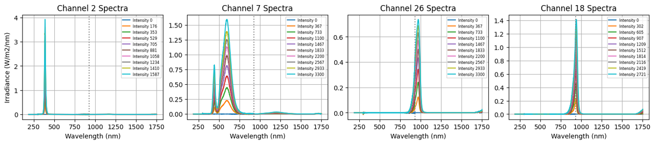
Fig. 4.25 Spectra acquired for individual channels of the G2V Pico at different intensity settings.

Representative results are shown in Figure 4.25. Channels 26 and 18 coincide with the spectrometer overlap region (900–1000 nm). Even here, the obtained spectra are smooth and free of stitching artifacts. The full dataset for all 32 channels is shown in Figure 4.26.

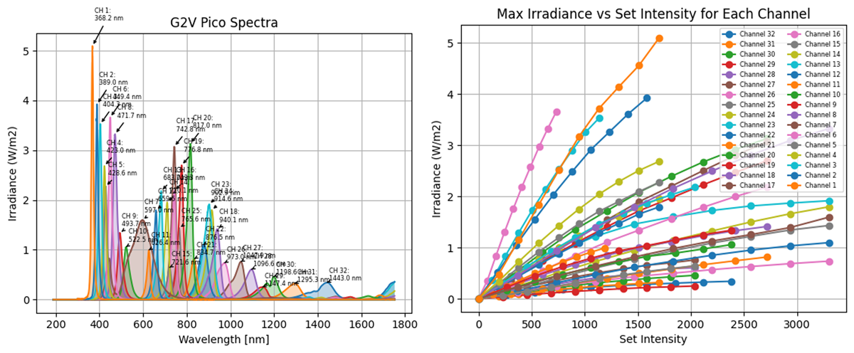
Fig. 4.26 Spectral distributions for all 32 channels of the G2V Pico (left) and the measured irradiance vs. intensity setpoint curves for each channel (right).

4.6.2.3. Simulating Solar Spectra

The recorded sensitivity data allows us to reconstruct any desired spectrum using multivariate optimization. Because physical LED channels cannot emit a negative amount of light, we formulate the reconstruction of the target spectrum as a constrained optimization problem—specifically, a bounded non-negative least squares (NNLS) problem. The optimizer finds the set of intensity settings that minimizes the residual sum of squares between the target spectrum and the calculated linear combination of the individual LED spectra, subject to the constraint that channel intensities must lie within \([0, I_{\max}]\). We then apply these optimized settings to the solar simulator hardware and verify the actual physical output using the dual-spectrometer setup.

Warning

It is essential to ensure that calculated intensity settings do not exceed the hardware limits of individual channels.

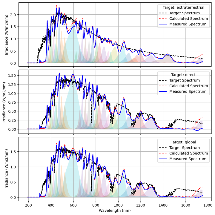
Fig. 4.27 Replicating ASTM G173-03 standard spectra based on the measured spectral distributions and sensitivity of each LED.

The results for the three ASTM G173-03 standards are shown in Figure 4.27. The filled areas represent the calculated output of each LED channel, the red line is the predicted sum, the black trace is the target, and the blue trace is the actual measurement.

• The calculated spectrum matches the target very well, which is significant given the complexity of optimizing 32 independent variables.

• The agreement between the predicted and measured spectra is excellent.

• Minor deviations (e.g., around 600 nm in the AM0 spectrum) are likely due to the total current limits of the solar simulator hardware.

Next, we used the SPECTRL2 model from pvlib to simulate the solar spectrum’s evolution throughout a day, accounting for:

• Solar position (location, date, time).

• Atmospheric conditions (elevation, azimuth, water vapor, turbidity).

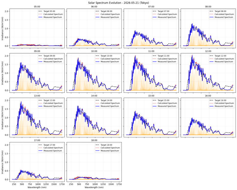
Fig. 4.28 Evolution of the solar spectrum during a simulated day in May in Tokyo.

Figure 4.28 shows the calculated spectrum from sunrise to sunset (black), the target intensity distribution (red), and the measured spectra (blue). The deviations observed in the blue spectral range during sunrise/sunset are likely due to non-linearities in the blue LEDs at very low intensity settings, which were not sufficiently captured during the initial characterization.

4.6.2.4. Simulating Stellar Spectra

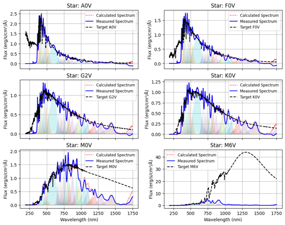
Fig. 4.29 Simulated spectra for different stellar classifications.

The G2V company name stems from the classification of our Sun as a G-type main-sequence star. The G2V Pico can also replicate spectra of other star types, albeit within its hardware constraints. Figure 4.29 displays simulations and measurements for:

• A0V (e.g., Vega): Surface temp. 7,600–10,000 K.

• F0V: Surface temp. 6,000–7,200 K.

• G2V (Sun-like): Surface temp. 5,300–6,000 K.

• K0V (Orange dwarf): Cooler than the Sun.

• M0V / M6V (Red dwarf/giant): Dominated by NIR emission.

For hot main-sequence stars like A0V, the broad-band shape in the visible range is well-approximated, though the ultraviolet (UV) region remains uncovered. Furthermore, narrow spectral features, such as the strong hydrogen Balmer absorption lines characteristic of A-type stars, cannot be resolved or replicated due to the relatively broad-band nature of the LED emitters. For cool, NIR-dominated M-class stars, although the spectral range matches the capability of the spectrometers, the absolute target irradiance is limited by the maximum optical output power of the simulator’s near-infrared LEDs.

4.6.2.5. Spectral Dashboard

Since both the G2V Pico and TII Spectrometry support TCP/IP control, it is straightforward to implement an interactive dashboard. This allows for:

• Real-time computation of solar spectra based on environmental parameters.

• Automated hardware configuration and spectral verification.

An example dashboard (built with iPython) is shown in Figure 4.30. Users can adjust date/time, detector tilt, atmospheric water, and turbidity. The dashboard streamlines the entire workflow—from calculation to hardware application and measurement—into a few clicks.

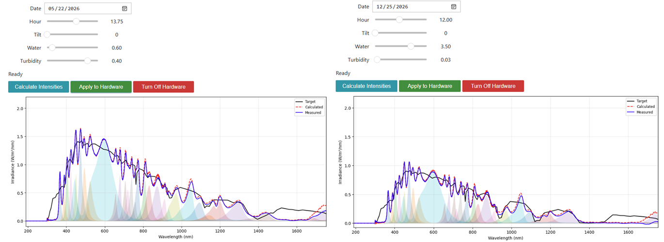
Fig. 4.30 An interactive dashboard for calculating, emitting, and verifying solar spectra.

Note

This dashboard serves as a prototype of how TII Spectrometry can eliminate friction in complex hardware orchestration. By handling device communication, synchronization, and calibration, it allows researchers to focus on the experiment rather than the data acquisition plumbing.

4.6.2.6. Closed-loop Spectral Simulations

Finally, we can implement a closed-loop feedback system. Instead of relying solely on pre-recorded sensitivity data, the system iteratively adjusts the LED intensities based on the actual measured spectrum to minimize the mismatch with the target.

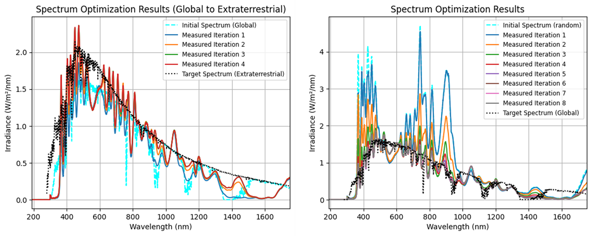
Fig. 4.31 Closed-loop spectral simulation. Left: Simulating the AM0 spectrum using AM1.5G as a starting point. Right: Simulating AM1.5G from random starting values. Solid lines show the emission after each optimization iteration.

As shown in Figure 4.31, the spectral mismatch decreases with each iteration, reaching excellent agreement with the target.

Note

While closed-loop optimization could theoretically work without prior knowledge, the 32 independent channels make it impractical. At each optimization step, the algorithm requires the Jacobian matrix \(J_{ij} = \partial S(\lambda_i) / \partial I_j\), representing the rate of change of the spectral irradiance \(S\) at wavelength \(\lambda_i\) with respect to the control setpoint \(I_j\) of the \(j\)-th LED. Evaluating this Jacobian experimentally at each iteration would require perturbing all 32 channels individually and acquiring 32 separate spectra, which is prohibitively slow.

Instead, by utilizing the pre-recorded individual channel calibration data, we can estimate this Jacobian analytically. This allows the gradient-based optimizer (such as a Levenberg-Marquardt or trust-region algorithm) to converge rapidly, requiring only a single spectrum acquisition per feedback loop iteration to correct for real-time drift, thermal effects, or electrical limitations. This approach is highly effective for:

• Accounting for complex non-linearities (cross-talk, thermal effects, current limits).

• Compensating for spectral drift due to LED aging.

• Cross-calibrating different solar simulator units.