
3.5. Kramers-Kronig Analysis#
The reflectance spectrum of a bulk sample does not look like its absorption spectrum. Near a strong absorption band, the reflectance depends on both the refractive index \(n\) and the extinction coefficient \(k\), so bands appear as derivative-like, dispersive features instead of clean peaks (Figure 3.22, panel A). This makes reflectance spectra difficult to interpret and to compare with library spectra measured in transmission or absorbance.
Kramers-Kronig analysis removes this distortion. It uses the fact that the real and imaginary parts of a causal optical response are not independent: the phase shift \(\theta(\nu)\) that light experiences on reflection can be calculated from the reflectance spectrum \(R(\nu)\) alone. Together, \(R(\nu)\) and \(\theta(\nu)\) determine the complex refractive index \(\tilde{N}(\nu) = n(\nu) + i\,k(\nu)\) and, from it, the absorption coefficient \(\alpha(\nu)\), which resembles an ordinary absorption spectrum.
TII Spectrometry performs this analysis on live spectra and on saved spectra. It is available for the following devices:
ARCoptix FTIR spectrometers
the NLIR Midwave
spectrometers that are combined with the NLIR Spectrum upconverter
For these devices, the menu contains the submenu.
See also
See Section 3.5.3 for a complete example using an ARCoptix FTIR spectrometer.
3.5.1. Method#
The analysis consists of the following steps:
A reflectance spectrum \(R(\nu)\) is measured (see Using Kramers-Kronig Analysis). Here, \(\nu\) is the wavenumber in \(\text{cm}^{-1}\).
Phase retrieval: The complex reflection coefficient of the sample is written as
(3.1)#\[ \tilde{r}(\nu) = \sqrt{R(\nu)}\,e^{i\theta(\nu)} \]The phase \(\theta(\nu)\) is calculated from the measured reflectance using the Kramers-Kronig relation
(3.2)#\[ \theta(\nu_0) = -\frac{\nu_0}{\pi}\,\mathcal{P}\!\int_0^{\infty} \frac{\ln R(\nu) - \ln R(\nu_0)}{\nu^2 - \nu_0^2}\,d\nu \]where \(\mathcal{P}\) denotes the Cauchy principal value. Subtracting \(\ln R(\nu_0)\) in the numerator removes the singularity of the integrand at \(\nu = \nu_0\) without changing the result, because \(\mathcal{P}\!\int_0^{\infty} d\nu / (\nu^2 - \nu_0^2) = 0\).
Fresnel inversion: For light at normal incidence, the Fresnel equations relate \(R\) and \(\theta\) to the optical constants of the sample:
(3.3)#\[ n(\nu) = \frac{1 - R(\nu)}{1 + R(\nu) - 2\sqrt{R(\nu)}\cos\theta(\nu)}, \qquad k(\nu) = \frac{2\sqrt{R(\nu)}\sin\theta(\nu)}{1 + R(\nu) - 2\sqrt{R(\nu)}\cos\theta(\nu)} \]Absorption coefficient: The (Napierian) absorption coefficient follows from the extinction coefficient:
(3.4)#\[ \alpha(\nu) = 4\pi\nu\,k(\nu) \]With \(\nu\) in \(\text{cm}^{-1}\), \(\alpha\) is also given in \(\text{cm}^{-1}\).
The integral in (3.2) extends from zero to infinity, but spectra cover only a finite range. To reduce truncation artifacts, TII Spectrometry evaluates the integral numerically (using the trapezoidal rule) on the measured wavenumber grid, extended on both ends by a constant continuation of the first and last measured reflectance value. The extension reaches down to zero wavenumber on the low side and to three times the highest measured wavenumber on the high side.
3.5.2. Using Kramers-Kronig Analysis#
3.5.2.1. Measuring reflectance#
Kramers-Kronig analysis requires the reflectance \(R\) as input. TII Spectrometry obtains it from the Transmittance display mode: the ratio of the sample spectrum to a reference spectrum, divided by 100, is interpreted as the reflectance. To measure a reflectance spectrum:
Record a reference spectrum using a reflectance standard, e.g. a mirror, in place of the sample.
Select Transmittance for the Y axis in the display settings.
Measure the sample under the same conditions.
The spectrum shown is now the reflectance of the sample relative to the reference.
Note
The display mode is called Transmittance because the same calculation is used for transmission measurements. When Kramers-Kronig analysis is used, the ratio is interpreted as a reflectance. The vertical axis of the reflectance spectrum in Figure 3.22 is therefore labeled Transmittance (%).
Important
The reflectance is calculated as the ratio to the reference spectrum. The reflectivity of the reference is assumed to be 100 %. If the reference does not fulfill this assumption, the reflectance of the sample and hence \(n\), \(k\) and \(\alpha\) are scaled accordingly.
3.5.2.2. Settings#
Kramers-Kronig analysis is configured in the submenu:
- Use
Toggles Kramers-Kronig analysis. The analysis is applied to the displayed spectrum immediately. It has no effect unless the Y axis is set to Transmittance.
- Mode
Selects the quantity that is displayed after the analysis:
N displays the refractive index \(n(\nu)\)
K displays the extinction coefficient \(k(\nu)\)
Absorption displays the absorption coefficient \(\alpha(\nu) = 4\pi\nu\,k(\nu)\) (default)
The label of the vertical axis changes accordingly.
Note
The phase \(\theta(\nu)\) is calculated as an intermediate result, but it cannot be selected for display.
Hint
Kramers-Kronig analysis can also be applied to saved spectra. Select the spectra in the sidebar and choose from the context menu. The analysis then uses the current settings of the submenu.
3.5.3. Example: Black PLA#
Figure 3.22 shows the analysis of the reflectance spectrum of a black PLA (polylactic acid) sample, recorded using an ARCoptix FTIR spectrometer.
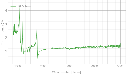
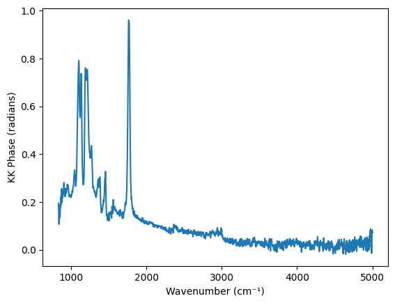
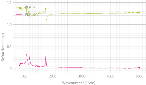
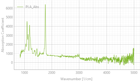
Fig. 3.22 Kramers-Kronig analysis of the reflectance spectrum of black PLA. Panel B shows the phase, which is an intermediate result. The refractive index \(n\) and extinction coefficient \(k\) (panel C) and the absorption coefficient (panel D) can be displayed using the Mode setting#
The panels show the steps of the analysis:
- A
The reflectance spectrum is low (about 1 % to 4 %) and dominated by dispersive features at the strong PLA bands: the C-O stretching bands between about \(1000\,\text{cm}^{-1}\) and \(1300\,\text{cm}^{-1}\) and the ester C=O stretching band at about \(1750\,\text{cm}^{-1}\). Between the bands, the reflectance is about 1.2 % to 1.4 %.
- B
The Kramers-Kronig relation (3.2) yields the phase \(\theta(\nu)\), which is largest at the strongest bands.
- C
Fresnel inversion (3.3) yields \(n\) and \(k\). Away from the bands, \(n\) is about 1.25, which is consistent with the reflectance of about 1.2 % to 1.4 % between the bands (\(R = \left(\frac{n-1}{n+1}\right)^2\) for \(k \approx 0\)). The refractive index shows the typical anomalous dispersion at the absorption bands, while \(k\) shows peaks at the band positions.
- D
The absorption coefficient (3.4) shows the PLA bands as regular absorption peaks. The noise increases towards high wavenumbers because \(k\) is multiplied by \(\nu\).
3.5.4. Notes and Limitations#
The analysis makes the following assumptions, which need to be considered when interpreting results:
- Sample and measurement geometry
The Fresnel equations (3.3) describe specular reflection at normal incidence from a flat, smooth surface of an optically thick (opaque) sample. Diffuse reflection from rough surfaces, light that is transmitted through the sample and reflected from its back side, and surface layers are not accounted for and will distort the result.
- Spectral range
Kramers-Kronig analysis is most accurate if the measured spectrum covers all strong absorption bands of the sample. The constant extension of the spectrum only partly compensates for bands outside of the measured range. Strong bands beyond the edges of the spectrum cause systematic errors, such as a sloping baseline or negative values of \(k\) and \(\alpha\).
- Noise
Noise in the reflectance spectrum propagates into the calculated phase and optical constants. Because the absorption coefficient is proportional to \(\nu\) ((3.4)), its noise increases towards higher wavenumbers (Figure 3.22, panel D). Averaging improves the result.
- Reflectance range
The reflectance is restricted to the range 0.0001 % to 99.99 % to avoid taking the logarithm of zero. Reflectance values of 100 % or more are not physical for a passive sample. They indicate a problem with the reference or the measurement, and the results are then not meaningful.
- Computation time
The analysis is repeated for every spectrum, and the required time increases with the square of the number of spectral points. In our tests, the calculation took about 0.06 s for 2000 points and about 0.6 s for 8000 points. For long spectra, this can limit the refresh rate during live acquisition. In this case, record the spectra first and apply the analysis afterwards using .